ncsim Documentation
| Description | Comprehensive guide to the Networked Compute Simulator |
| Repository | https://github.com/ANRGUSC/ncsim |
| Copyright | Copyright © 2026 Autonomous Networks Research Group (ANRG), University of Southern California |
ncsim Documentation
ncsim (Networked Compute Simulator) is a headless discrete-event simulator for evaluating task scheduling algorithms on heterogeneous networked systems. It models compute nodes, network links with WiFi interference, and DAG task graphs, producing detailed JSONL traces and JSON metrics for analysis.
Developed by the Autonomous Networks Research Group (ANRG) at the University of Southern California.
Key Features
- Deterministic simulation -- same inputs plus the same seed produce identical results every time
- HEFT / CPOP / Round Robin scheduling -- integrated with anrg-saga schedulers, plus manual task pinning
- Multi-hop routing -- direct, widest-path (max-min bandwidth), and shortest-path (min-latency) algorithms
- 802.11 WiFi PHY/MAC modeling -- log-distance path loss, SNR-based MCS rate adaptation for 802.11n/ac/ax
- Interference models -- none, proximity, CSMA/CA clique-based, and CSMA/CA Bianchi (dynamic SINR)
- Fair bandwidth sharing -- concurrent transfers on the same link share capacity proportionally
- Web visualization UI -- interactive experiment builder, Gantt charts, animated replay, and network topology views
- Structured output -- JSONL event traces and JSON summary metrics for automated analysis
Guide Roadmap
This documentation is organized into eight sections, each covering a different aspect of ncsim:
| # | Section | What You Will Learn |
|---|---|---|
| 1 | Getting Started | Install ncsim, its dependencies, and the optional visualization frontend |
| 2 | Core Concepts | Understand the architecture, simulation model, scheduling, routing, and interference |
| 3 | Scenarios | Write and customize YAML scenario files that define networks, DAGs, and configurations |
| 4 | CLI Usage | Run simulations from the command line, interpret output files, and automate batch experiments |
| 5 | Visualization | Set up and use the web UI to configure experiments and explore results interactively |
| 6 | Experiments | Reproduce interference verification and routing comparison experiments |
| 7 | Tutorials | Follow step-by-step walkthroughs from first simulation to advanced WiFi experiments |
| 8 | Reference | Look up FAQs, troubleshooting tips, and the glossary |
New to ncsim?
Start with the Installation guide, then follow the Quick Start to run your first simulation in under five minutes.
Quick Links
-
Installation
Set up Python, clone the repository, and install all dependencies.
-
Quick Start
Run your first simulation and examine the output in five minutes.
-
Scenario YAML Reference
Full specification of nodes, links, DAGs, tasks, and config options.
-
CLI Reference
All command-line flags, overrides, and usage examples.
-
Visualization
Interactive web UI for building scenarios and exploring results.
-
Tutorials
Guided walkthroughs from basic to advanced usage.
How It Works
At a high level, ncsim follows this pipeline:
graph LR
    A[Scenario YAML] --> B[Scenario Loader]
    B --> C[Scheduler<br/>HEFT / CPOP / RR]
    C --> D[Simulation Engine]
    D --> E[Trace JSONL]
    D --> F[Metrics JSON]
    F --> G[Viz UI / Analysis]
E --> G- You define a scenario in YAML: network topology, node capacities, link bandwidths, DAG task graphs, and configuration (scheduler, routing, interference model, seed).
- The scheduler (powered by anrg-saga) assigns tasks to nodes.
- The simulation engine executes the schedule as a discrete-event simulation, modeling compute time, data transfers, multi-hop routing, bandwidth sharing, and WiFi interference.
- The engine produces a JSONL trace (every event) and JSON metrics (summary statistics including makespan, utilization).
- You can analyze the output with the included
analyze_trace.pyscript, feed it into the web visualization UI, or process it with your own tools.
Project Information
| Repository | github.com/ANRGUSC/ncsim |
| PyPI package | anrg-ncsim |
| License | MIT |
| Python | 3.10+ |
| Contributors | Bhaskar Krishnamachari, Maya Gutierrez |
| Organization | Autonomous Networks Research Group (ANRG), University of Southern California |
Citation
If you use ncsim in your research, please cite it. See the CITATION.cff file in the repository for the recommended citation format.
Getting Started
Installation
This guide walks through installing ncsim, its dependencies, and the optional web visualization frontend.
Prerequisites
Verify that the following tools are installed and meet the minimum version requirements:
| Tool | Minimum Version | Check Command | Notes |
|---|---|---|---|
| Python | 3.10+ | python --version |
Required |
| pip | 21+ | pip --version |
Required |
| Git | 2.30+ | git --version |
Required for cloning the repo |
| Node.js | 18+ | node --version |
Viz frontend only |
| npm | 9+ | npm --version |
Viz frontend only |
Node.js is optional
Node.js and npm are only required if you plan to use the web visualization UI. The core simulator and CLI work with just Python.
Clone the Repository
The recommended way to get started is to clone the full repository. This gives you the example scenarios, experiment scripts, documentation, and web visualization UI:
Install ncsim
Editable Install (Recommended)
Install ncsim in editable (development) mode so that changes to the source code take effect immediately:
This installs the following dependencies automatically:
| Package | Version | Purpose |
|---|---|---|
| anrg-saga | >= 2.0.3 | HEFT, CPOP, and Round Robin scheduling algorithms |
| networkx | >= 3.0 | Graph data structures for routing and conflict graphs |
| pyyaml | >= 6.0 | YAML scenario file parsing |
To also install development dependencies (pytest, pytest-cov), use:
PyPI Install (Core Only)
Alternatively, install just the core simulator package from PyPI:
PyPI install does not include extras
The pip install anrg-ncsim command installs only the core simulator library and the ncsim CLI. It does not include the example scenarios, experiment scripts, visualization UI, or documentation. Use this option if you want to integrate ncsim as a library in your own project and will write your own scenario YAML files.
Verify the CLI
After installation, confirm that the ncsim command is available:
Expected output:
Install the Visualization Backend
The visualization backend is a FastAPI server that connects the web UI to ncsim. Install its dependencies from the viz/server/ directory:
This installs:
| Package | Version | Purpose |
|---|---|---|
| FastAPI | >= 0.115.0 | REST API framework |
| uvicorn | >= 0.34.0 | ASGI server |
Install the Visualization Frontend
The frontend is a React application built with Vite. Install its Node.js dependencies:
Stay in the project root
After running npm install, return to the project root directory so that subsequent ncsim commands work with the correct relative paths to scenario files.
Verify the Installation
Verify the CLI
Run the included demo_simple scenario to confirm the simulator works end to end:
You should see output ending with:
=== Simulation Complete ===
Scenario: Simple Demo
Scheduler: heft
Routing: direct
Interference: proximity
  radius=15.0
Seed: 42
Makespan: 3.000000 seconds
Total events: 7
Status: completed
Confirm that three output files were created:
Verify the Visualization
Start the backend and frontend in two separate terminals:
Open http://localhost:5173 in your browser. You should see the ncsim-viz interface with a Configure & Run panel.
Run the Test Suite
To run the full test suite and confirm everything is functioning correctly:
Or equivalently:
The test suite includes unit tests for the event queue, execution engine, scheduling, routing, WiFi physics, interference models, and end-to-end acceptance tests.
Troubleshooting
1. ModuleNotFoundError: No module named 'ncsim'
Cause: ncsim is not installed in your current Python environment.
Fix: Run pip install -e . from the repository root. If you are using a virtual environment, make sure it is activated first.
# Activate your virtual environment (if using one)
source venv/bin/activate    # Linux/macOS
venv\Scripts\activate       # Windows

# Install ncsim
pip install -e .
2. ncsim: command not found
Cause: The pip scripts directory is not on your system PATH.
Fix: Either add pip's script directory to your PATH, or invoke ncsim as a Python module:
# Option A: Run as a module
python -m ncsim --scenario scenarios/demo_simple.yaml --output results/test

# Option B: Find and add the scripts directory
python -m site --user-base
# Add the bin/ (Linux/macOS) or Scripts/ (Windows) subdirectory to your PATH
3. Frontend shows "Network Error" when running an experiment
Cause: The FastAPI backend server is not running, or it is running on a different port than expected.
Fix: Start the backend in a separate terminal:
Confirm it is listening on http://localhost:8000 before using the frontend.
4. Port 8000 or 5173 is already in use
Cause: Another process is occupying the port.
Fix: Find and stop the conflicting process, or run on a different port:
5. npm install fails with errors
Cause: Node.js version is too old. The frontend requires Node.js 18 or later.
Fix: Update Node.js to version 18+ and try again:
node --version    # Check current version

# Update using your package manager, nvm, or download from https://nodejs.org/
nvm install 18    # If using nvm
npm install       # Retry
6. Visualization shows no experiments / empty experiment list
Cause: The viz/public/sample-runs/ directory is missing or contains no experiment results.
Fix: Run a simulation with output directed to the sample-runs directory, or copy an existing results folder there:
Then refresh the visualization in your browser.
7. ImportError: cannot import name ... from 'saga'
Cause: The anrg-saga package is not installed, or an incompatible version is installed.
Fix: Install or upgrade anrg-saga to version 2.0.3 or later:
If you have a different package named saga installed, it may conflict. Uninstall it first:
Next Steps
With ncsim installed, head to the Quick Start guide to run your first simulation in under five minutes.
Quick Start
Run your first ncsim simulation in five minutes. This guide assumes you have already completed the Installation steps.
Step 1: Run Your First Simulation
The repository includes several example scenarios in the scenarios/ directory. Start with the simplest one -- a two-node network with a two-task DAG:
You should see the following terminal output:
=== Simulation Complete ===
Scenario: Simple Demo
Scheduler: heft
Routing: direct
Interference: proximity
  radius=15.0
Seed: 42
Makespan: 3.000000 seconds
Total events: 7
Status: completed
What just happened?
ncsim loaded the scenario, used the HEFT scheduler to assign two tasks to nodes, ran a discrete-event simulation, and produced output files with the full event trace and summary metrics. The makespan (3.0 seconds) is the total time from the start of the first task to the completion of the last task.
Step 2: Examine the Output Files
Every simulation run produces three files in the output directory:
| File | Format | Contents |
|---|---|---|
scenario.yaml |
YAML | Copy of the input scenario (for reproducibility) |
trace.jsonl |
JSONL | Every simulation event, one JSON object per line |
metrics.json |
JSON | Summary metrics: makespan, utilization, task/transfer counts |
Trace File (trace.jsonl)
The trace file records every event in chronological order. Each line is a self-contained JSON object with a sequence number, simulation time, and event type:
{"sim_time":0.0,"type":"sim_start","trace_version":"1.0","seed":42,"scenario":"demo_simple.yaml","seq":0}
{"sim_time":0.0,"type":"dag_inject","dag_id":"dag_1","task_ids":["T0","T1"],"seq":1}
{"sim_time":0.0,"type":"task_scheduled","dag_id":"dag_1","task_id":"T0","node_id":"n0","seq":2}
{"sim_time":0.0,"type":"task_start","dag_id":"dag_1","task_id":"T0","node_id":"n0","seq":3}
{"sim_time":1.0,"type":"task_complete","dag_id":"dag_1","task_id":"T0","node_id":"n0","duration":1.0,"seq":4}
{"sim_time":1.0,"type":"task_scheduled","dag_id":"dag_1","task_id":"T1","node_id":"n0","seq":5}
{"sim_time":1.0,"type":"task_start","dag_id":"dag_1","task_id":"T1","node_id":"n0","seq":6}
{"sim_time":3.0,"type":"task_complete","dag_id":"dag_1","task_id":"T1","node_id":"n0","duration":2.0,"seq":7}
{"sim_time":3.0,"type":"sim_end","status":"completed","makespan":3.0,"total_events":8,"seq":8}
The event types you will encounter are:
| Event Type | Description |
|---|---|
sim_start |
Simulation begins; records scenario name, seed, trace version |
dag_inject |
A DAG is injected into the simulation with its list of task IDs |
task_scheduled |
A task is assigned to a specific node by the scheduler |
task_start |
A task begins executing on its assigned node |
task_complete |
A task finishes executing; includes duration |
transfer_start |
A data transfer begins between tasks across a link |
transfer_complete |
A data transfer finishes; includes duration |
sim_end |
Simulation ends; records final status and makespan |
Metrics File (metrics.json)
The metrics file provides a high-level summary of the simulation run:
{
  "scenario": "demo_simple.yaml",
  "seed": 42,
  "makespan": 3.0,
  "total_tasks": 2,
  "total_transfers": 1,
  "total_events": 7,
  "status": "completed",
  "node_utilization": {
    "n0": 1.0,
    "n1": 0.0
  },
  "link_utilization": {
    "l01": 0.0
  }
}
Utilization
Node utilization is the fraction of the makespan during which a node is actively executing a task. Link utilization is the fraction of the makespan during which a link is carrying data. In this example, HEFT assigned both tasks to node n0, so n0 has 100% utilization, n1 has 0%, and link l01 was never used.
Step 3: Override Settings from the CLI
Scenario YAML files define default settings (scheduler, routing, seed), but you can override any of them from the command line. Try running the same scenario with a different scheduler, routing algorithm, and seed:
ncsim --scenario scenarios/demo_simple.yaml --output results/demo-cpop \
      --scheduler cpop --routing widest_path --seed 123
=== Simulation Complete ===
Scenario: Simple Demo
Scheduler: cpop
Routing: widest_path
Interference: proximity
  radius=15.0
Seed: 123
Makespan: 3.000000 seconds
Total events: 7
Status: completed
In this simple two-node case, both HEFT and CPOP produce the same makespan because the optimal strategy is to run both tasks on the faster node. The differences become significant on larger topologies.
The full set of CLI overrides:
| Flag | Values | Description |
|---|---|---|
--scheduler |
heft, cpop, round_robin, manual |
Scheduling algorithm |
--routing |
direct, widest_path, shortest_path |
Routing algorithm |
--interference |
none, proximity, csma_clique, csma_bianchi |
Interference model |
--interference-radius |
float | Radius for proximity interference (meters) |
--seed |
integer | Random seed for deterministic results |
--wifi-standard |
n, ac, ax |
WiFi standard for MCS rate tables |
--tx-power |
float (dBm) | WiFi transmit power |
--freq |
float (GHz) | WiFi carrier frequency |
--path-loss-exponent |
float | Path loss exponent |
--rts-cts |
flag | Enable RTS/CTS mechanism |
--verbose / -v |
flag | Enable debug-level logging |
Step 4: Try a More Complex Scenario
The parallel_spread.yaml scenario demonstrates the impact of routing on a multi-node topology. It defines 5 nodes in a line with 8 parallel tasks:
=== Simulation Complete ===
Scenario: Parallel Spread (Bidirectional)
Scheduler: heft
Routing: direct
Interference: proximity
  radius=15.0
Seed: 42
Makespan: 35.348333 seconds
Total events: 51
Status: completed
Now run the same scenario with widest-path routing, which enables the scheduler to spread tasks across all 5 nodes via multi-hop paths:
=== Simulation Complete ===
Scenario: Parallel Spread (Bidirectional)
Scheduler: heft
Routing: widest_path
Interference: proximity
  radius=15.0
Seed: 42
Makespan: 24.246722 seconds
Total events: 55
Status: completed
31% faster with widest-path routing
With direct routing, HEFT can only assign tasks to nodes that have a direct link to the task's data source, limiting it to 3 adjacent nodes. Widest-path routing enables multi-hop transfers, so HEFT can spread the 8 parallel tasks across all 5 nodes -- reducing the makespan from 35.3s to 24.2s.
Step 5: Analyze the Trace
The included analyze_trace.py script provides quick text-based analysis of trace files. Use the --timeline flag for a chronological event log and --gantt flag for an ASCII Gantt chart:
=== Event Timeline ===

[  0.0000] sim_start            scenario=demo_simple.yaml
[  0.0000] dag_inject           dag=dag_1, tasks=['T0', 'T1']
[  0.0000] task_scheduled       T0 on n0
[  0.0000] task_start           T0 on n0
[  1.0000] task_complete        T0 on n0 (duration=1.0)
[  1.0000] task_scheduled       T1 on n0
[  1.0000] task_start           T1 on n0
[  3.0000] task_complete        T1 on n0 (duration=2.0)
[  3.0000] sim_end              makespan=3.0

=== Execution Gantt Chart ===

Time: 0                                                        3.00s
       |============================================================|
n0     |####################                                        | T0 (1.000s)
n0     |                    ########################################| T1 (2.000s)
       |============================================================|

Legend: # = task execution, ~ = data transfer
The analysis script supports three views:
| Flag | Description |
|---|---|
--timeline |
Chronological event log with timestamps |
--gantt |
ASCII Gantt chart showing task execution and data transfers |
--tasks |
Per-task detail: scheduled time, start time, completion time, duration, wait time |
You can combine flags, or run with no flags to get a default summary plus Gantt chart.
What's Next?
Now that you have run your first simulations, explore the rest of the documentation:
- Core Concepts: Architecture -- understand the simulation engine, event queue, and execution model
- Core Concepts: Scheduling -- learn how HEFT, CPOP, and Round Robin assign tasks to nodes
- Scenarios: YAML Reference -- full specification of the scenario file format for writing your own scenarios
- Scenarios: Scenario Gallery -- browse the 10 included example scenarios with descriptions and expected results
- Visualization: Overview -- set up the web UI and explore results interactively with Gantt charts, animated replay, and network topology views
- Tutorial 2: Custom Scenario -- build a scenario from scratch
- Tutorial 3: WiFi Experiment -- configure 802.11 interference models
- Tutorial 4: Compare Schedulers -- run batch experiments comparing scheduling algorithms
Core Concepts
Architecture
ncsim is a headless discrete event simulator for networked computing, designed around pluggable abstractions for scheduling, routing, and interference modeling. This page describes the package structure, data flow, key abstractions, and the optional visualization frontend.
Package Structure
ncsim/
├── main.py             # CLI entry point (argparse, orchestration)
├── core/
│   ├── simulation.py   # Main simulation loop (Simulation, SimulationResult)
│   ├── event_queue.py  # Priority queue with deterministic ordering
│   ├── execution_engine.py  # Event handlers, node/link state management
│   └── telemetry.py    # Pluggable telemetry collectors
├── models/
│   ├── network.py      # Node, Link, Position, Network dataclasses
│   ├── task.py         # Task, TaskState, TaskStatus, FIFOQueueModel
│   ├── dag.py          # DAG, Edge, DAGSource ABC
│   ├── routing.py      # RoutingModel ABC + 3 implementations
│   ├── interference.py # InterferenceModel ABC + 4 implementations
│   └── wifi.py         # 802.11 RF physics (PHY rates, conflict graph, Bianchi)
├── scheduler/
│   ├── base.py         # Scheduler ABC, PlacementPlan, RoundRobinScheduler
│   └── saga_adapter.py # HEFT/CPOP via anrg-saga library
└── io/
    ├── scenario_loader.py  # YAML parsing -> Scenario object
    ├── trace_writer.py     # JSONL trace output (event stream)
    └── results_writer.py   # metrics.json output (summary)
Architecture Overview
The high-level data flow follows a linear pipeline from YAML input through simulation to structured output files.
flowchart LR
    YAML["Scenario YAML"] --> SL["ScenarioLoader"]
    SL --> SIM["Simulation"]
    SIM --> TW["TraceWriter"]
    SIM --> RW["ResultsWriter"]
    TW --> TRACE["trace.jsonl"]
    RW --> METRICS["metrics.json"]
Simulation Pipeline
The simulation proceeds through seven distinct phases. Each phase transforms or consumes the output of the previous one.
flowchart TD
    A["1. Load<br/>ScenarioLoader reads YAML<br/>-> Scenario with Network, DAGs, Config"] --> B
    B["2. Configure<br/>CLI overrides applied<br/>(--scheduler, --routing, --interference, --seed)"] --> C
    C["3. Wire<br/>Simulation constructed with<br/>Scheduler, DAGSource,<br/>RoutingModel, InterferenceModel"] --> D
    D["4. Inject<br/>DAGs injected at inject_at times<br/>Scheduler returns PlacementPlan<br/>for each DAG"] --> E
    E["5. Execute<br/>Event loop: pop from priority queue<br/>ExecutionEngine handles each event<br/>New events scheduled as side effects"] --> F
    F["6. Trace<br/>Events forwarded to TraceWriter<br/>-> trace.jsonl (one JSON object per line)"] --> G
    G["7. Results<br/>Makespan, utilization, status<br/>-> metrics.json"]
Phase Details
1. Load. The ScenarioLoader reads a YAML file and produces a
Scenario object containing a Network (nodes + links), a list of
DAG objects (tasks + edges), and a ScenarioConfig with defaults for
scheduler, routing, interference, and seed.
2. Configure. CLI arguments such as --scheduler heft,
--routing widest_path, or --interference csma_bianchi override the
values from the YAML config section. The --seed flag overrides the
scenario seed for reproducibility experiments.
3. Wire. The Simulation object is constructed, which internally
creates an EventQueue and an ExecutionEngine. The engine receives
handles to the Network, Scheduler, RoutingModel, and optionally an
InterferenceModel.
4. Inject. The DAGSource (either SingleDAGSource or
MultiDAGSource) provides DAGs at their specified inject_at times. For
each DAG, a DAG_INJECT event is placed on the queue. When that event is
processed, the scheduler's on_dag_inject method is called, returning a
PlacementPlan that maps every task to a node.
5. Execute. The main loop pops events from the priority queue one at a
time. Each event is dispatched to the appropriate handler in the
ExecutionEngine, which may schedule new events as side effects. The loop
continues until the queue is empty.
6. Trace. A TraceEventAdapter listens to every processed event and
writes structured records to a JSONL file via TraceWriter. Each record
includes a sequence number, simulation time, event type, and
event-specific fields.
7. Results. After the loop completes, the ResultsWriter computes
makespan, per-node utilization, per-link utilization, and simulation
status, then writes everything to metrics.json.
Key Abstractions
ncsim uses abstract base classes (ABCs) at every extension point. Swapping behavior requires only implementing the ABC and selecting it via CLI flag or YAML config.
| Abstraction | Interface | Implementations | Configured by |
|---|---|---|---|
| Scheduler | on_dag_inject(dag, snapshot) -> PlacementPlan |
RoundRobinScheduler, ManualScheduler, SagaScheduler (HEFT, CPOP) |
--scheduler |
| RoutingModel | get_path(src, dst, network) -> [link_ids] |
DirectLinkRouting, WidestPathRouting, ShortestPathRouting |
--routing |
| InterferenceModel | get_interference_factor(link, actives, net) -> float |
NoInterference, ProximityInterference, CsmaCliqueInterference, CsmaBianchiInterference |
--interference |
| DAGSource | get_next_injection(after_time) -> (time, dag) |
SingleDAGSource, MultiDAGSource |
Scenario YAML |
| TelemetryCollector | on_event(event, engine) |
TraceOnlyCollector, FullStateCollector |
Internal |
| QueueModel | enqueue(task), dequeue() -> task |
FIFOQueueModel |
Internal |
Scheduler
The scheduler decides where tasks run. It receives a DAG and a
NetworkSnapshot (read-only view of nodes and links with capacities and
bandwidths), and returns a PlacementPlan mapping every task ID to a node
ID. The execution engine decides when tasks run based on event
ordering and node availability.
Pinned tasks
Any task with a pinned_to field in the YAML overrides the
scheduler's assignment. This works with all schedulers, including
HEFT and CPOP.
RoutingModel
The routing model determines the path (sequence of link IDs) for
data transfers between nodes. DirectLinkRouting requires an explicit
link and fails if none exists. WidestPathRouting finds the path that
maximizes bottleneck bandwidth using modified Dijkstra. ShortestPathRouting
minimizes total latency using standard Dijkstra.
InterferenceModel
The interference model computes a multiplicative factor in (0, 1] applied
to a link's base bandwidth when other links are simultaneously active.
This is orthogonal to per-link fair sharing: if a link has base bandwidth
B, interference factor f, and N concurrent transfers, each transfer gets
(B * f) / N.
DAGSource
A DAGSource provides DAGs for injection into the simulation at specified
times. SingleDAGSource injects one DAG. MultiDAGSource injects
multiple DAGs sorted by their inject_at times.
Extensibility
Adding new models
To add a new scheduling algorithm, routing model, or interference model, implement the corresponding ABC and register it in the CLI argument choices and factory function.
The ABC-based architecture supports the following future extensions without modifying the core simulation loop:
- RL-based scheduling -- Implement
Scheduler.on_dag_injectwith a trained policy network. - Preemptive tasks -- Extend
QueueModelwith priority-based preemption; theTaskStatealready trackscompute_remaining. - TDMA links -- Implement a
LinkModelthat returns time-varying bandwidth based on slot schedules. TheEventTypeenum already reservesTDMA_SLOT_START. - Mobility -- Schedule
MOBILITY_UPDATEevents that recompute positions and update link bandwidths. The event type is already reserved. - Jamming / disruptions -- Schedule
LINK_STATE_CHANGEevents that degrade or disable links mid-simulation.
Visualization Architecture
ncsim includes an optional web-based visualization frontend (viz/
directory) for interactive trace playback and scenario editing.
Stack
| Layer | Technology |
|---|---|
| Frontend | React 19, TypeScript, Vite |
| Layout & graphics | D3.js (network graph), Dagre (DAG layout) |
| Styling | Tailwind CSS 4 |
| Backend | FastAPI + uvicorn (Python) |
| Simulation | ncsim invoked as subprocess |
Communication
The frontend development server (Vite, port 5173) proxies all /api/*
requests to the FastAPI backend running on port 8000. The backend
accepts scenario YAML, runs ncsim as a subprocess, and returns the
parsed trace and metrics to the browser.
sequenceDiagram
    participant Browser
    participant FastAPI
    participant ncsim

    Browser->>FastAPI: POST /api/run {yaml}
    FastAPI->>ncsim: subprocess.run(["ncsim", ...])
    ncsim-->>FastAPI: trace.jsonl, metrics.json
    FastAPI-->>Browser: {scenario, trace, metrics}
The browser receives the full simulation output in a single response and renders an interactive timeline with network topology, DAG structure, and event-by-event playback.
Simulation Model
ncsim uses a discrete event simulation (DES) to model task execution and data transfer across a networked computing environment. This page covers the event model, time management, compute and transfer calculations, and bandwidth sharing mechanics.
Discrete Event Simulation Basics
A discrete event simulation advances time by jumping from one event to the next, rather than stepping through fixed time increments. The core loop is:
- Pop the highest-priority event from the queue.
- Advance the simulation clock to that event's time.
- Execute the event handler, which may schedule new events.
- Repeat until the queue is empty.
No fixed time step
Unlike tick-based simulations, DES skips idle periods entirely. A simulation with two events at t=0.0 and t=100.0 processes only those two events, regardless of the 100-second gap between them.
This approach gives ncsim exact timing for task completions and data transfers without discretization error.
Event Types
ncsim defines six core event types, each with a fixed priority value. Lower priority values are processed first when multiple events occur at the same simulation time.
| Event Type | Priority | Description |
|---|---|---|
DAG_INJECT |
0 | A new DAG arrives and is handed to the scheduler |
TASK_COMPLETE |
1 | A task finishes execution on its assigned node |
TRANSFER_COMPLETE |
2 | A data transfer finishes on its link path |
TASK_READY |
3 | All predecessors of a task are satisfied |
TASK_START |
4 | A task begins execution on a node |
TRANSFER_START |
5 | A data transfer begins on a link |
Why completions come before starts
At the same simulation time, completions must be processed before starts. When a task completes, it frees its node and triggers output transfers. Those transfers may complete instantly (same-node), making a downstream task ready. If starts were processed first, the downstream task could miss being scheduled at the correct time.
Four additional event types are reserved for future extensions:
MOBILITY_UPDATE (100), LINK_STATE_CHANGE (101),
RESCHEDULE_TRIGGER (102), and TDMA_SLOT_START (103). Their handlers
currently no-op.
Event Ordering
Events are stored in a min-heap (priority queue) and ordered by a three-element sort key:
| Component | Purpose |
|---|---|
round(sim_time, 6) |
Microsecond precision avoids floating-point comparison issues |
event_type.priority |
Ensures correct causal ordering at the same time instant |
event_id |
Monotonically increasing counter guarantees FIFO order for ties |
This three-level ordering guarantees determinism: given the same inputs and the same seed, the simulation produces an identical event sequence every time.
Event Cancellation
The queue supports lazy cancellation. When a transfer's completion time is recalculated (due to bandwidth sharing changes), the old completion event is added to a cancelled set. When the queue pops a cancelled event, it silently discards it and pops the next one. This avoids the cost of heap removal while maintaining correctness.
Determinism
Reproducibility guarantee
Same scenario YAML + same --seed = identical event sequence,
identical makespan, identical trace output.
Determinism comes from three sources:
- Microsecond rounding -- All times are rounded to 6 decimal places
via
round_time(), eliminating platform-dependent floating-point drift. - Priority-based ordering -- Event type priorities impose a fixed processing order at each time instant.
- Monotonic event IDs -- A global counter breaks all remaining ties in insertion order.
Compute Model
Each node has a compute_capacity measured in compute units per second.
Each task has a compute_cost measured in compute units. The execution
time is:
For example, a task with compute_cost: 200 on a node with
compute_capacity: 100 takes 2.0 seconds.
Node Queuing
Each node runs at most one task at a time (single-server model). When a task becomes ready and its assigned node is busy, the task enters a FIFO queue on that node. Tasks are dequeued and started in arrival order when the node becomes idle.
No preemption
A running task always completes before any queued task starts. The
TaskState dataclass tracks compute_remaining to support future
preemptive scheduling, but the current engine does not interrupt
running tasks.
Task Lifecycle
A task moves through these statuses:
| Status | Meaning |
|---|---|
PENDING |
Waiting for predecessor tasks to complete |
READY |
All predecessors complete; waiting for node availability |
QUEUED |
In the node's FIFO queue (node is busy) |
RUNNING |
Executing on the node |
COMPLETED |
Finished execution |
Transfer Model
When a task completes, the engine schedules data transfers for each outgoing edge in the DAG. Transfers move data from the source task's node to the destination task's node over a network path.
Local Transfers
If the source and destination tasks are assigned to the same node, no network transfer occurs. The predecessor is marked complete immediately at zero cost.
Network Transfers
For tasks on different nodes, the routing model determines a path (sequence of link IDs). The transfer time is:
Where:
data_sizeis the edge'sdata_sizein MB.effective_bandwidthis the bottleneck bandwidth across all links in the path, after accounting for per-link fair sharing and interference.total_latencyis the sum of all link latencies along the path (store-and-forward model).
Multi-Hop Paths
For paths with more than one link:
- Bottleneck bandwidth = minimum bandwidth across all links in the path.
- Total latency = sum of latencies across all links (each hop adds its propagation delay).
The store-and-forward model means data must fully arrive at each intermediate node before being forwarded to the next hop.
Bandwidth Sharing
When multiple transfers use the same link simultaneously, they share the
link's bandwidth equally. If N transfers share a link with base bandwidth
B (after interference), each gets B / N.
Dynamic recalculation
When a transfer starts or completes on a link, the engine recalculates the completion times of all other active transfers on that link. Old completion events are cancelled and replaced with new ones reflecting the updated bandwidth allocation.
The recalculation accounts for partial progress. When bandwidth changes mid-transfer:
- The engine computes how much data was transferred at the previous rate during the elapsed time.
- It subtracts that from
data_remaining. - It schedules a new completion event based on the remaining data and the new effective rate.
For multi-hop transfers, the effective bandwidth is the minimum across all links in the path, each independently sharing its bandwidth among its concurrent transfers.
Interference Effects on Bandwidth
When an InterferenceModel is active, bandwidth sharing becomes a
two-level calculation:
- Interference factor: The model returns a factor f in (0, 1] for each link based on other active links in the network (e.g., nearby wireless transmitters).
- Per-link fair sharing: N concurrent transfers on the link each get
(B * f) / N.
Interference factors are recomputed whenever any transfer starts or completes, and affected transfers have their completion times recalculated.
Example: Two-Task Execution
The following diagram shows the event sequence for a simple scenario with two tasks (T0 and T1) where T1 depends on T0 and they are assigned to different nodes.
sequenceDiagram
    participant EQ as Event Queue
    participant Engine as ExecutionEngine

    Note over EQ,Engine: t=0.000000
    EQ->>Engine: DAG_INJECT (dag_1)
    Note right of Engine: Scheduler assigns T0->n0, T1->n1<br/>Schedules TASK_READY for root task T0

    EQ->>Engine: TASK_READY (T0)
    Note right of Engine: Node n0 is idle<br/>Schedules TASK_START for T0

    EQ->>Engine: TASK_START (T0, n0)
    Note right of Engine: runtime = 100 / 100 = 1.0s<br/>Schedules TASK_COMPLETE at t=1.0

    Note over EQ,Engine: t=1.000000
    EQ->>Engine: TASK_COMPLETE (T0, n0)
    Note right of Engine: T0 done. Edge T0->T1 has data_size=50 MB<br/>T0 on n0, T1 on n1: network transfer<br/>Schedules TRANSFER_START

    EQ->>Engine: TRANSFER_START (T0->T1, link l01)
    Note right of Engine: effective_bw = 100 MB/s, latency = 0.001s<br/>transfer_time = 50/100 + 0.001 = 0.501s<br/>Schedules TRANSFER_COMPLETE at t=1.501

    Note over EQ,Engine: t=1.501000
    EQ->>Engine: TRANSFER_COMPLETE (T0->T1)
    Note right of Engine: T1's last predecessor satisfied<br/>Schedules TASK_READY for T1

    EQ->>Engine: TASK_READY (T1)
    Note right of Engine: Node n1 is idle<br/>Schedules TASK_START for T1

    EQ->>Engine: TASK_START (T1, n1)
    Note right of Engine: runtime = 200 / 50 = 4.0s<br/>Schedules TASK_COMPLETE at t=5.501

    Note over EQ,Engine: t=5.501000
    EQ->>Engine: TASK_COMPLETE (T1, n1)
    Note right of Engine: No successors. DAG complete.<br/>Makespan = 5.501000s
Tracing this locally
Run this exact scenario with:
The verbose flag (-v) logs every event to the console. The
output directory will contain trace.jsonl and metrics.json.
Output Files
trace.jsonl
One JSON object per line, in event order. Every record has:
| Field | Type | Description |
|---|---|---|
seq |
int | Monotonically increasing sequence number |
sim_time |
float | Simulation time in seconds (6 decimal places) |
type |
string | Event type (dag_inject, task_start, task_complete, transfer_start, transfer_complete, sim_start, sim_end) |
Additional fields vary by event type (e.g., dag_id, task_id,
node_id, link_id, duration, data_size).
metrics.json
A single JSON object with summary metrics:
| Field | Type | Description |
|---|---|---|
scenario |
string | Scenario file name |
seed |
int | Random seed used |
makespan |
float | Time of last task completion |
total_tasks |
int | Number of tasks across all DAGs |
total_transfers |
int | Number of data transfer edges |
total_events |
int | Total events processed |
status |
string | "completed" or "error" |
node_utilization |
object | Per-node busy_time / makespan (0.0 to 1.0) |
link_utilization |
object | Per-link data_transferred / (bandwidth * makespan) |
Scheduling Algorithms
ncsim supports three scheduling algorithms that decide where each
task runs. The scheduler receives a DAG and a snapshot of the network
(node capacities, link bandwidths), and returns a PlacementPlan
mapping every task to a node. The execution engine then decides
when tasks run based on event ordering and node availability.
Select a scheduler via CLI:
Or in the scenario YAML:
HEFT (Heterogeneous Earliest Finish Time)
HEFT is a list-scheduling heuristic designed for heterogeneous computing environments. It is the default scheduler in ncsim and generally produces the best makespans.
Algorithm
-
Compute upward rank for each task. The upward rank is the longest path (by computation + communication cost) from the task to any exit task in the DAG. Tasks with higher upward rank are scheduled first.
-
Sort tasks by decreasing upward rank. This ordering ensures that tasks on the critical path are considered before less important tasks.
-
For each task (in rank order), evaluate every node and select the one that gives the earliest finish time (EFT). The finish time accounts for:
- The task's execution time on that node (
compute_cost / compute_capacity). - The data transfer time for all incoming edges from predecessor tasks already placed on other nodes.
- The node's availability (when it becomes idle after finishing its currently assigned workload).
- The task's execution time on that node (
Communication awareness
HEFT accounts for the cost of data transfers between nodes. If two communicating tasks are placed on the same node, the transfer cost is zero. This means HEFT will naturally co-locate tightly coupled tasks when the communication cost outweighs the benefit of faster remote execution.
When to Use HEFT
- General-purpose default for heterogeneous networks.
- Networks where nodes have different compute capacities.
- DAGs with mixed computation and communication requirements.
CPOP (Critical Path on a Processor)
CPOP is a variant of list scheduling that identifies the DAG's critical path and concentrates those tasks on the single fastest processor.
Algorithm
-
Compute upward rank and downward rank for each task. The downward rank is the longest path from the entry task to the current task.
-
Compute priority as the sum of upward and downward rank. Tasks on the critical path all share the same maximum priority value.
-
Identify critical-path tasks -- tasks whose priority equals the maximum.
-
Assign critical-path tasks to the single processor (node) that minimizes the total critical-path execution time.
-
Assign non-critical tasks using the EFT heuristic (same as HEFT).
When to Use CPOP
- DAGs with a dominant critical path (one long chain of dependent tasks).
- Networks with one node significantly faster than the others, where running the critical path entirely on that node avoids inter-node transfer overhead.
CPOP can underperform HEFT
If the DAG has multiple paths of similar length, CPOP's strategy of concentrating on a single critical path may leave the fast processor overloaded while other nodes sit idle. In such cases, HEFT's per-task EFT approach tends to produce better makespans.
Round Robin
Round Robin assigns tasks to nodes in simple cyclic order. It is communication-unaware and heterogeneity-unaware.
Algorithm
- Order tasks topologically (predecessors before successors).
- Cycle through nodes: task 0 goes to node 0, task 1 to node 1, task 2 to node 0, and so on.
Baseline only
Round Robin ignores compute capacities, data dependencies, and transfer costs. It exists solely as a baseline for comparing against intelligent schedulers. Do not use it for performance- sensitive simulations.
Comparison
| Feature | HEFT | CPOP | Round Robin |
|---|---|---|---|
| Task ordering | Upward rank (descending) | Priority = upward + downward rank | Topological (insertion order) |
| Node selection | Earliest Finish Time (EFT) across all nodes | Critical-path tasks to fastest node; others to min EFT | Cyclic assignment |
| Communication-aware | Yes | Yes | No |
| Heterogeneity-aware | Yes | Yes | No |
| Best for | General case | Dominant critical path + one fast node | Baseline comparisons |
| Library | anrg-saga | anrg-saga | Built-in |
Manual Assignment (pinned_to)
Tasks can be pinned to specific nodes using the pinned_to field in the
scenario YAML. This bypasses the scheduler's decision for that task.
dags:
  - id: dag_1
    tasks:
      - id: T0
        compute_cost: 100
        pinned_to: n0        # Force T0 onto node n0
      - id: T1
        compute_cost: 200
        pinned_to: n1        # Force T1 onto node n1
      - id: T2
        compute_cost: 150    # No pin -- scheduler decides
    edges:
      - { from: T0, to: T2, data_size: 10 }
      - { from: T1, to: T2, data_size: 20 }
Pinned tasks work with any scheduler:
- With
--scheduler manual, all tasks must havepinned_toset (tasks without it are assigned to the first node with a warning). - With
--scheduler heftor--scheduler cpop, pinned tasks override the scheduler's choice. Unpinned tasks are scheduled normally. - With
--scheduler round_robin, pinned tasks override the cyclic assignment.
Testing specific placements
Manual assignment is useful for validating simulation correctness against hand-calculated expected results, or for testing how a specific placement performs under different interference or routing models.
Example: Same DAG, Different Schedulers
Consider a diamond-shaped DAG with four tasks on a two-node network:
scenario:
  name: "Diamond DAG"
  network:
    nodes:
      - id: fast
        compute_capacity: 100
      - id: slow
        compute_capacity: 50
    links:
      - id: link_fs
        from: fast
        to: slow
        bandwidth: 10
        latency: 0.001
      - id: link_sf
        from: slow
        to: fast
        bandwidth: 10
        latency: 0.001

  dags:
    - id: diamond
      tasks:
        - { id: A, compute_cost: 100 }   # Entry
        - { id: B, compute_cost: 200 }   # Left branch
        - { id: C, compute_cost: 200 }   # Right branch
        - { id: D, compute_cost: 100 }   # Exit (merge)
      edges:
        - { from: A, to: B, data_size: 5 }
        - { from: A, to: C, data_size: 5 }
        - { from: B, to: D, data_size: 5 }
        - { from: C, to: D, data_size: 5 }
HEFT Placement
HEFT computes upward ranks and assigns each task to the node giving the earliest finish time:
| Task | Upward Rank | Assignment | Rationale |
|---|---|---|---|
| A | highest | fast | Fastest execution for the entry task |
| B | mid | fast | Co-locating with A avoids transfer cost |
| C | mid | slow | Runs in parallel with B on the other node |
| D | lowest | fast | Fastest node for the exit merge |
Because B and C can run in parallel on different nodes, HEFT overlaps their execution. The makespan is dominated by the critical path A -> B -> D (or A -> C -> D, whichever is longer after accounting for transfer times).
CPOP Placement
CPOP identifies the critical path (e.g., A -> B -> D) and assigns all
three to fast. Task C (non-critical) goes to slow via EFT.
| Task | On Critical Path | Assignment |
|---|---|---|
| A | Yes | fast |
| B | Yes | fast |
| C | No | slow |
| D | Yes | fast |
This avoids transfers along the critical path (A, B, D all on the same node), but C must transfer its output to D across the network.
Round Robin Placement
Round Robin simply cycles: A -> fast, B -> slow, C -> fast, D -> slow.
| Task | Assignment | Rationale |
|---|---|---|
| A | fast | First in cycle |
| B | slow | Second in cycle |
| C | fast | Third in cycle (wraps) |
| D | slow | Fourth in cycle |
This placement is communication-unaware. Every edge in the DAG requires a network transfer, and the slow node bottlenecks task execution. The resulting makespan is significantly worse than HEFT or CPOP.
Makespan Comparison
Running the three schedulers on the diamond scenario above produces different makespans. The exact values depend on bandwidth and latency parameters, but the relative ranking is consistent:
# Run with each scheduler
ncsim --scenario diamond.yaml --output out/heft --scheduler heft
ncsim --scenario diamond.yaml --output out/cpop --scheduler cpop
ncsim --scenario diamond.yaml --output out/rr   --scheduler round_robin
| Scheduler | Typical Makespan Ranking |
|---|---|
| HEFT | Best (parallelism + communication-aware) |
| CPOP | Close to HEFT (critical path optimized) |
| Round Robin | Worst (no optimization) |
SAGA Library Integration
HEFT and CPOP are implemented via the
anrg-saga library. ncsim's
SagaScheduler adapter translates between ncsim's data model and SAGA's:
-
Network translation -- SAGA requires a fully-connected graph. The adapter creates edges for all node pairs:
LOCAL_SPEED(10000 MB/s) for same-node, actual link bandwidth for connected pairs, widest-path bandwidth for multi-hop pairs (when--routing widest_pathor--routing shortest_pathis active), andDISCONNECTED_SPEED(0.001 MB/s) for unreachable pairs. -
Task graph translation -- DAG tasks become
TaskGraphNodeobjects withcost = compute_cost. DAG edges becomeTaskGraphEdgeobjects withsize = data_size. -
Result extraction -- SAGA's schedule maps internal node names (
node_0,node_1) to task lists. The adapter maps these back to actual node IDs.
Routing Modes
ncsim supports three routing modes that determine how data flows between nodes
in the network. The routing mode is set via the routing key in the scenario
YAML or the --routing CLI flag.
Direct Routing (direct)
Single-hop routing that transfers data only on a direct link between the source and destination nodes.
- No multi-hop: if no direct link exists between two nodes, the transfer fails immediately.
- Simplest and fastest: no path computation, no caching overhead.
- Best for: topologies where every communicating pair of nodes has a dedicated link.
Transfer failure
Direct routing will fail any transfer where the source and destination
are not connected by a single declared link. If your scheduler may assign
communicating tasks to non-adjacent nodes, use widest_path or
shortest_path instead.
Widest Path Routing (widest_path)
Routes data along the path that maximizes the bottleneck bandwidth (max-min bandwidth). This is the optimal choice when transfer size dominates total transfer time.
- Algorithm: modified Dijkstra using a max-heap. At each step the
algorithm relaxes edges by taking
min(current_bottleneck, link_bandwidth), keeping the path whose minimum-bandwidth link is largest. - Multi-hop: intermediate nodes act as store-and-forward relays.
- Caching: paths are computed once and cached for the lifetime of the
simulation. Call
clear_cache()if the topology changes. - Transfer model: bottleneck bandwidth determines transfer rate; latencies are summed across all hops (store-and-forward).
Shortest Path Routing (shortest_path)
Routes data along the path that minimizes total latency (sum of per-link latencies). When all links have equal latency this degenerates to minimum hop count.
- Algorithm: standard Dijkstra on link latencies (min-heap).
- Multi-hop: intermediate nodes act as store-and-forward relays.
- Caching: paths are computed once and cached.
- Transfer model: latencies are summed; bottleneck bandwidth along the chosen path determines transfer rate.
Comparison
| Feature | Direct | Widest Path | Shortest Path |
|---|---|---|---|
| Algorithm | Direct lookup | Modified Dijkstra (max-min BW) | Standard Dijkstra (min latency) |
| Multi-hop | No | Yes | Yes |
| Optimizes | N/A | Bottleneck bandwidth | Total latency |
| Fails when | No direct link exists | No path exists | No path exists |
| Path caching | N/A | Yes | Yes |
| Best for | Simple topologies | Large transfers | Small / latency-sensitive transfers |
When Widest and Shortest Diverge
The two multi-hop modes choose different paths whenever a topology offers a trade-off between bandwidth and latency. Consider a diamond topology with two relay nodes:
graph LR
    src -- "BW=20 MB/s<br/>lat=0.001s" --> relay_fast
    relay_fast -- "BW=20 MB/s<br/>lat=0.001s" --> dst
    src -- "BW=200 MB/s<br/>lat=0.05s" --> relay_wide
    relay_wide -- "BW=200 MB/s<br/>lat=0.05s" --> dst

    style relay_fast fill:#cce5ff,stroke:#004085
    style relay_wide fill:#d4edda,stroke:#155724
Shortest path picks src -> relay_fast -> dst (total latency 0.002 s,
bottleneck BW 20 MB/s).
Widest path picks src -> relay_wide -> dst (total latency 0.1 s,
bottleneck BW 200 MB/s).
Worked Example -- 100 MB Transfer
This corresponds to the widest_vs_shortest.yaml scenario, where tasks T0
(on src) and T1 (on dst) are connected by a 100 MB data edge. Each task
has compute_cost: 100 on nodes with compute_capacity: 100, so each task
takes 1.0 s to execute.
| Shortest Path | Widest Path | |
|---|---|---|
| Path | src -> relay_fast -> dst | src -> relay_wide -> dst |
| Bottleneck BW | 20 MB/s | 200 MB/s |
| Total latency | 0.002 s | 0.1 s |
| Transfer time | 100 / 20 + 0.002 = 5.002 s | 100 / 200 + 0.1 = 0.6 s |
| Makespan | 1.0 + 5.002 + 1.0 = 7.002 s | 1.0 + 0.6 + 1.0 = 2.6 s |
Widest-path routing is approximately 2.7x faster for this large transfer because the data volume dominates the total time, making bandwidth the controlling factor.
Rule of thumb
Use widest_path when transfer sizes are large relative to link
latencies. Use shortest_path when transfers are small and latency
dominates.
When Multi-hop Routing Is Needed
Why multi-hop matters
Multi-hop routing is required whenever the scheduler assigns communicating
tasks to non-adjacent nodes -- that is, nodes with no direct link
between them. Without widest_path or shortest_path routing, the
transfer will fail because direct routing cannot relay through
intermediate nodes.
This commonly occurs with HEFT and CPOP schedulers, which choose node assignments based on compute speed and may place dependent tasks on nodes that are not directly connected.
YAML Configuration
Routing is specified in the config section:
Or overridden on the command line:
Interference Models
Interference models reduce the effective bandwidth of a link when multiple
nearby links are simultaneously active. This inter-link contention is applied
on top of per-link fair sharing (where N flows on the same link each get
bandwidth / N).
The combined formula for a single flow on a link is:
The interference model is selected via the interference key in the scenario
YAML or the --interference CLI flag.
None (none)
No inter-link interference. The interference factor is always 1.0.
- Links operate at their full declared bandwidth regardless of concurrent transfers on other links.
- Appropriate for wired networks or scenarios where spectrum contention is not relevant.
Proximity (proximity)
A simple distance-based interference model. Links whose geometric midpoints fall within a configurable radius are considered to be contending.
- If k active links (including the link being evaluated) have midpoints
within the radius, the interference factor is
1/k. - Configure the radius with the
interference_radiusYAML key or the--interference-radiusCLI flag (default: 15.0 meters). - Dynamic: the factor is recalculated whenever a transfer starts or completes.
- Provides a quick approximation of spectrum contention without requiring WiFi-specific RF parameters.
CSMA/CA Clique (csma_clique)
An 802.11-aware static model that builds a conflict graph based on carrier sensing rules and divides bandwidth by the worst-case clique size.
- Uses RF propagation (path loss, carrier sensing threshold) to determine which links can sense each other's transmissions.
- Links that can sense each other form edges in a conflict graph. The Bron-Kerbosch algorithm (exact for networks with 50 or fewer links; greedy approximation otherwise) finds the maximum clique containing each link.
-
At setup time, each link's bandwidth is set to:
-
After setup, the interference factor is always 1.0 -- contention is baked into the bandwidth value and does not change during simulation.
- Conservative: represents the worst-case bound where all links in the largest clique transmit simultaneously.
- Requires RF parameters (
tx_power_dBm,freq_ghz,path_loss_exponent,cca_threshold_dBm, etc.) via therf:YAML section.
CSMA/CA Bianchi (csma_bianchi)
The most realistic WiFi interference model. It dynamically separates two distinct interference mechanisms:
1. Contention Domain (Conflict Graph Neighbors)
Links that appear as neighbors in the conflict graph operate under CSMA/CA: they cannot transmit simultaneously. Instead, they share airtime according to Bianchi's saturation throughput model.
Each of n contending links (including the link itself) gets a fraction
eta(n) / n of the channel, where eta(n) is the Bianchi MAC efficiency
for n stations.
Because CSMA prevents simultaneous transmission, contending links do not cause SINR degradation at each other's receivers.
2. Hidden Terminals (Non-Conflict-Graph Neighbors)
Active links that are not in the conflict graph of the evaluated link may transmit simultaneously, causing RF interference at the receiver. Their combined interference power degrades the SINR, which may force a lower MCS rate.
The SINR-based rate (R_SINR) is computed using only hidden terminal
interference. The base rate (R_base) is the SNR-only PHY rate.
Combined Factor
Where:
n = 1 + |active contending neighbors|eta(n)= Bianchi MAC efficiency for n stationsR_SINR= MCS rate under SINR (hidden terminal degradation)R_base= MCS rate under SNR only (no interference)
The factor is recalculated whenever a transfer starts or completes, making this a fully dynamic model.
config:
  interference: csma_bianchi
  rf:
    tx_power_dBm: 20
    freq_ghz: 5.0
    path_loss_exponent: 3.0
    noise_floor_dBm: -95
    cca_threshold_dBm: -82
    channel_width_mhz: 20
    wifi_standard: "ax"
Key insight
CSMA prevents simultaneous transmission within the contention domain, so
contending links affect throughput via time-sharing, not via SINR
degradation. Only hidden terminals -- links outside the conflict graph --
contribute to SINR reduction. This separation is what distinguishes
csma_bianchi from simpler models.
Comparison
| Feature | None | Proximity | CSMA Clique | CSMA Bianchi |
|---|---|---|---|---|
| Interference type | None | Distance-based | Carrier sensing | SINR + MAC |
| Dynamic | N/A | Yes | No (static) | Yes |
| WiFi-aware | No | No | Yes | Yes |
| RF parameters required | No | No | Yes | Yes |
| Accuracy | N/A | Low | Medium | High |
| Use case | Wired networks | Quick approximation | WiFi without SINR | Realistic WiFi |
Worked Example: Proximity Interference
This example uses the interference_test.yaml scenario.
Topology
Four nodes with two parallel links, 5 units apart:
graph LR
    n0["n0 (0,0)"] -- "l01: BW=100 MB/s" --> n1["n1 (5,0)"]
n2["n2 (0,5)"] -- "l23: BW=100 MB/s" --> n3["n3 (5,5)"]- Link
l01midpoint: (2.5, 0) - Link
l23midpoint: (2.5, 5) - Distance between midpoints: 5.0 units
Two DAG edges create simultaneous transfers: T0 -> T1 on l01 (100 MB) and
T2 -> T3 on l23 (100 MB). Each task has compute_cost: 10 on nodes with
compute_capacity: 1000, so task execution takes 0.01 s.
Without Interference (none)
| Transfer | Bandwidth | Time | Total |
|---|---|---|---|
| T0 -> T1 on l01 | 100 MB/s | 100 / 100 = 1.0 s | 0.01 + 1.0 + 0.01 = 1.02 s |
| T2 -> T3 on l23 | 100 MB/s | 100 / 100 = 1.0 s | 0.01 + 1.0 + 0.01 = 1.02 s |
Makespan: 1.02 s
With Proximity Interference (radius=10)
Since the midpoint distance (5.0) is less than the radius (10.0), both links
contend. With k=2 active contending links, the interference factor is 1/k = 0.5.
| Transfer | Effective BW | Time | Total |
|---|---|---|---|
| T0 -> T1 on l01 | 100 * 0.5 = 50 MB/s | 100 / 50 = 2.0 s | 0.01 + 2.0 + 0.01 = 2.02 s |
| T2 -> T3 on l23 | 100 * 0.5 = 50 MB/s | 100 / 50 = 2.0 s | 0.01 + 2.0 + 0.01 = 2.02 s |
Makespan: 2.02 s -- transfers take 2x longer due to interference.
YAML Configuration
Proximity Model
WiFi Models (Clique or Bianchi)
config:
  interference: csma_bianchi   # or csma_clique
  rf:
    tx_power_dBm: 20
    freq_ghz: 5.0
    path_loss_exponent: 3.0
    noise_floor_dBm: -95
    cca_threshold_dBm: -82
    channel_width_mhz: 20
    wifi_standard: "ax"
    shadow_fading_sigma: 0.0
    rts_cts: false
CLI Overrides
WiFi Model
The WiFi model replaces manually specified link bandwidths with physically
grounded data rates derived from RF propagation, SNR-based MCS selection,
and 802.11 MAC contention. It is used by the csma_clique and csma_bianchi
interference models.
The implementation lives in two modules:
ncsim/models/wifi.py-- RF propagation, MCS tables, conflict graph construction, Bianchi MAC efficiencyncsim/models/interference.py--CsmaCliqueInterferenceandCsmaBianchiInterferenceclasses
Path Loss and Received Power
ncsim uses the log-distance path loss model with a Friis free-space reference at distance d0 = 1 m.
Friis Reference Loss
The free-space path loss at the reference distance d0:
At 5 GHz with d0 = 1 m, this evaluates to approximately 46.4 dB. At 2.4 GHz with d0 = 1 m, approximately 40.0 dB.
Log-Distance Path Loss
For distance d >= d0:
Where n is the path loss exponent:
| Environment | Typical n |
|---|---|
| Free space | 2.0 |
| Indoor (open office) | 2.5 - 3.0 |
| Indoor (with walls) | 3.0 - 4.0 |
| Dense indoor | 4.0 - 5.0 |
Received Power
Where X_SF is the shadow fading component (0 by default, see
Shadow Fading below).
SNR
Signal-to-noise ratio in dB:
Where N0 is the noise floor (default -95 dBm).
MCS Rate Adaptation
The received SNR selects the highest MCS (Modulation and Coding Scheme) whose minimum SNR threshold is met. If the SNR falls below 5 dB (the lowest threshold), the link is considered not viable and the rate is 0.
MCS Tables (1 Spatial Stream, 20 MHz Base)
802.11n (HT)
| MCS | Modulation | Min SNR (dB) | Rate (Mbps) |
|---|---|---|---|
| 0 | BPSK 1/2 | 5 | 6.5 |
| 1 | QPSK 1/2 | 8 | 13.0 |
| 2 | QPSK 3/4 | 11 | 19.5 |
| 3 | 16-QAM 1/2 | 14 | 26.0 |
| 4 | 16-QAM 3/4 | 18 | 39.0 |
| 5 | 64-QAM 2/3 | 22 | 52.0 |
| 6 | 64-QAM 3/4 | 25 | 58.5 |
| 7 | 64-QAM 5/6 | 29 | 65.0 |
802.11ac (VHT)
| MCS | Modulation | Min SNR (dB) | Rate (Mbps) |
|---|---|---|---|
| 0 | BPSK 1/2 | 5 | 6.5 |
| 1 | QPSK 1/2 | 8 | 13.0 |
| 2 | QPSK 3/4 | 11 | 19.5 |
| 3 | 16-QAM 1/2 | 14 | 26.0 |
| 4 | 16-QAM 3/4 | 18 | 39.0 |
| 5 | 64-QAM 2/3 | 22 | 52.0 |
| 6 | 64-QAM 3/4 | 25 | 58.5 |
| 7 | 64-QAM 5/6 | 29 | 65.0 |
| 8 | 256-QAM 3/4 | 32 | 78.0 |
| 9 | 256-QAM 5/6 | 35 | 86.7 |
802.11ax (HE)
| MCS | Modulation | Min SNR (dB) | Rate (Mbps) |
|---|---|---|---|
| 0 | BPSK 1/2 | 5 | 8.6 |
| 1 | QPSK 1/2 | 8 | 17.2 |
| 2 | QPSK 3/4 | 11 | 25.8 |
| 3 | 16-QAM 1/2 | 14 | 34.4 |
| 4 | 16-QAM 3/4 | 18 | 51.6 |
| 5 | 64-QAM 2/3 | 22 | 68.8 |
| 6 | 64-QAM 3/4 | 25 | 77.4 |
| 7 | 64-QAM 5/6 | 29 | 86.0 |
| 8 | 256-QAM 3/4 | 32 | 103.2 |
| 9 | 256-QAM 5/6 | 35 | 114.7 |
| 10 | 1024-QAM 3/4 | 38 | 129.0 |
| 11 | 1024-QAM 5/6 | 41 | 143.4 |
Summary by Standard
| Standard | MCS Range | Peak Rate (20 MHz) | Modulation Range |
|---|---|---|---|
| 802.11n | 0--7 | 65.0 Mbps | BPSK -- 64-QAM |
| 802.11ac | 0--9 | 86.7 Mbps | BPSK -- 256-QAM |
| 802.11ax | 0--11 | 143.4 Mbps | BPSK -- 1024-QAM |
Channel Width Scaling
Rates scale linearly with channel width. The table values are for 20 MHz; multiply by the channel width factor:
| Channel Width | Factor |
|---|---|
| 20 MHz | 1x |
| 40 MHz | 2x |
| 80 MHz | 4x |
| 160 MHz | 8x |
For example, 802.11ax MCS 11 at 80 MHz: 143.4 * 4 = 573.6 Mbps.
Unit Conversion
ncsim uses MB/s internally for bandwidth. PHY rates are converted:
Conflict Graph
The conflict graph determines which links cannot transmit simultaneously under the 802.11 CSMA/CA protocol model.
Carrier Sensing Range
The maximum distance at which a transmission triggers Clear Channel Assessment (CCA):
Where theta_CCA is the CCA threshold (default -82 dBm).
Conflict Rules
Two links A and B conflict if carrier sensing prevents them from transmitting at the same time.
Without RTS/CTS (default): links A and B conflict if:
- Transmitter of A can sense any node of link B, OR
- Transmitter of B can sense any node of link A
"Can sense" means the distance between the two nodes is within the carrier sensing range.
With RTS/CTS (rts_cts: true): links A and B conflict if:
- Any node of link A can sense any node of link B
RTS/CTS extends the conflict zone to protect receivers, which reduces hidden terminal problems but increases contention.
graph TB
    subgraph "Without RTS/CTS"
        direction LR
        txA1["TX(A)"] -->|"sense?"| txB1["TX(B)"]
        txA1 -->|"sense?"| rxB1["RX(B)"]
        txB1 -->|"sense?"| txA1b["TX(A)"]
        txB1 -->|"sense?"| rxA1["RX(A)"]
    end

    subgraph "With RTS/CTS"
        direction LR
        txA2["TX(A)"] -->|"sense?"| txB2["TX(B)"]
        txA2 -->|"sense?"| rxB2["RX(B)"]
        rxA2["RX(A)"] -->|"sense?"| txB2b["TX(B)"]
        rxA2 -->|"sense?"| rxB2b["RX(B)"]
    end
Max Clique Computation
For each link, ncsim computes the maximum clique size -- the largest set of mutually conflicting links that includes the given link.
- Exact (Bron-Kerbosch with pivoting): used when the network has 50 or fewer links. Finds all maximal cliques and records the largest one containing each link.
- Greedy approximation: used for larger networks. Builds a clique greedily starting from each link by adding the most-connected candidate that is adjacent to all current clique members.
Bianchi MAC Efficiency
Bianchi's saturation throughput model computes the MAC-layer efficiency
eta(n) for n contending stations sharing the channel under 802.11 DCF.
Coupled Equations
The model solves for the transmission probability tau and collision
probability p via fixed-point iteration:
Where:
- W = 16 (CWmin, minimum contention window for 802.11)
- m = 6 (maximum backoff stage; CWmax = W * 2^m = 1024)
Efficiency Values
From the converged tau and p, the model computes idle, success, and
collision probabilities per slot, then derives the fraction of channel time
carrying successful payload:
| n (stations) | eta(n) | Per-station share eta(n)/n |
|---|---|---|
| 1 | 1.000 | 1.000 |
| 2 | ~0.88 | ~0.44 |
| 5 | ~0.72 | ~0.14 |
| 10 | ~0.59 | ~0.059 |
| 20 | ~0.47 | ~0.024 |
Properties:
eta(1) = 1.0-- a single station has no contention overhead.eta(n)is monotonically decreasing but always positive.- The per-station share
eta(n)/ndecreases faster than1/ndue to collision overhead.
ncsim precomputes a lookup table for n = 1 to 100 at startup.
CSMA Clique Model
The static WiFi interference model. Contention is computed once at setup and baked into each link's bandwidth.
Bandwidth Assignment
Where omega(l) is the maximum clique size containing link l.
Interference Factor
Always 1.0. Since contention is already reflected in the bandwidth, the interference model does not apply any additional reduction during simulation.
When To Use
csma_clique is appropriate when you want WiFi-aware bandwidth estimation
without the computational cost of dynamic recalculation. It provides a
conservative worst-case bound: the bandwidth assumes all links in the
largest clique are always active, even if only a subset actually transmits
at any given time.
CSMA Bianchi Model
The dynamic WiFi interference model. It correctly separates two interference mechanisms and recalculates the factor whenever transfers start or complete.
Mechanism 1: Contention Domain Time-Sharing
Links that are neighbors in the conflict graph operate under CSMA/CA and cannot transmit simultaneously. Each of n contending links gets:
No SINR degradation occurs from these links because CSMA prevents concurrent transmission.
Mechanism 2: Hidden Terminal SINR Degradation
Active links that are not in the conflict graph may transmit simultaneously, causing interference at the receiver. The SINR is computed in the linear domain:
Where P_interferers includes only hidden terminal transmitter powers as
received at the evaluated link's receiver node. The SINR determines a
(potentially lower) MCS rate R_SINR.
Combined Factor
The factor is clamped to the range [0.01, 1.0].
Recalculation
When any transfer starts or completes, all other active links have their factors recalculated. This ensures both contention domain changes and hidden terminal changes are captured symmetrically.
flowchart TD
    A["Transfer starts/completes on link L"] --> B["Identify active links"]
    B --> C["For each active link K != L"]
    C --> D["Classify neighbors:<br/>contending vs. hidden"]
    D --> E["Compute contention_factor = eta(n)/n"]
    D --> F["Compute SINR from hidden terminals"]
    F --> G["Select MCS from SINR -> R_SINR"]
    E --> H["factor = (R_SINR / R_base) * (eta(n) / n)"]
    G --> H
    H --> I["Recalculate transfer completion time"]
Key design decision
Contending links affect throughput via time-sharing (Bianchi), not via SINR. Only hidden terminals cause SINR degradation. Conflating the two (e.g., including contending links in the SINR calculation) would double-count their impact and produce unrealistically low throughput.
Shadow Fading
Optional log-normal shadow fading adds randomness to path loss. In the dB domain, fading values are drawn from a Gaussian distribution N(0, sigma).
- Per-node-pair: each pair of nodes gets its own fading value.
- Symmetric: fading(A, B) = fading(B, A).
- Deterministic from seed: the same seed always produces the same fading map, ensuring reproducibility.
- Configured via
shadow_fading_sigma(default 0.0, meaning no fading).
The fading value is subtracted from received power:
Where X_SF ~ N(0, sigma) for the specific node pair.
RF Configuration Parameters
All RF parameters are specified in the rf: section of the scenario YAML.
Several can also be overridden via CLI flags.
| YAML Key | CLI Flag | Unit | Default | Description |
|---|---|---|---|---|
tx_power_dBm |
--tx-power |
dBm | 20.0 | Transmit power (typical AP: 15--23 dBm) |
freq_ghz |
--freq |
GHz | 5.0 | Carrier frequency (2.4 or 5.0) |
path_loss_exponent |
--path-loss-exponent |
-- | 3.0 | Path loss exponent n (2.0 = free space, 3--4 = indoor) |
noise_floor_dBm |
-- | dBm | -95.0 | Effective noise floor including receiver noise figure |
cca_threshold_dBm |
-- | dBm | -82.0 | CCA signal detect threshold |
channel_width_mhz |
-- | MHz | 20 | Channel width (20, 40, 80, 160) |
wifi_standard |
--wifi-standard |
-- | ax |
MCS table selection (n, ac, ax) |
shadow_fading_sigma |
-- | dB | 0.0 | Std dev of log-normal shadow fading (0 = none) |
rts_cts |
--rts-cts |
-- | false |
Enable RTS/CTS (extends conflict zone) |
Full YAML Example
config:
  interference: csma_bianchi
  rf:
    tx_power_dBm: 20
    freq_ghz: 5.0
    path_loss_exponent: 3.0
    noise_floor_dBm: -95
    cca_threshold_dBm: -82
    channel_width_mhz: 20
    wifi_standard: "ax"
    shadow_fading_sigma: 0.0
    rts_cts: false
Omitting link bandwidth
When using csma_clique or csma_bianchi, link bandwidth is derived
from RF parameters and node positions. You can omit the bandwidth key
from link definitions -- ncsim will compute it automatically. If you do
specify a bandwidth, it will be kept as-is (not overwritten by the WiFi
model), which is useful for mixing wired and wireless links in the same
topology.
CLI Override Example
Scenarios
YAML Reference
This page documents every field available in an ncsim scenario YAML file, with a complete annotated example and a field-by-field reference table.
Complete Annotated Example
The following YAML shows every supported field with inline comments explaining its purpose:
scenario:
  name: "My Experiment"

  network:
    nodes:
      - id: n0
        compute_capacity: 100      # compute units per second
        position: {x: 0, y: 0}     # meters (for interference and viz)
      - id: n1
        compute_capacity: 50
        position: {x: 10, y: 0}

    links:
      - id: l01
        from: n0                    # directional: n0 -> n1
        to: n1
        bandwidth: 100              # MB/s
        latency: 0.001              # seconds

  dags:
    - id: dag_1
      inject_at: 0.0               # simulation time to inject
      tasks:
        - id: T0
          compute_cost: 100         # compute units (runtime = cost / capacity)
          pinned_to: n0             # optional: force task to this node
        - id: T1
          compute_cost: 200
      edges:
        - from: T0
          to: T1
          data_size: 50             # MB

  config:
    scheduler: heft                 # heft | cpop | round_robin
    seed: 42
    routing: direct                 # direct | widest_path | shortest_path
    interference: proximity         # none | proximity | csma_clique | csma_bianchi
    interference_radius: 15.0       # meters (proximity model only)
    rf:                             # WiFi models only
      tx_power_dBm: 20
      freq_ghz: 5.0
      path_loss_exponent: 3.0
      noise_floor_dBm: -95
      cca_threshold_dBm: -82
      channel_width_mhz: 20
      wifi_standard: ax
      shadow_fading_sigma: 0
      rts_cts: false
Field-by-Field Reference
Scenario Root
| Field | Type | Required | Default | Description |
|---|---|---|---|---|
scenario.name |
string | No | File stem | Human-readable name for the scenario. Used in CLI output and result metadata. |
Nodes (scenario.network.nodes[])
| Field | Type | Required | Default | Description |
|---|---|---|---|---|
nodes[].id |
string | Yes | -- | Unique identifier for the node. Referenced by links, pinned_to, and routing. |
nodes[].compute_capacity |
float | Yes | -- | Processing speed in compute units per second. Task runtime = compute_cost / compute_capacity. |
nodes[].position |
object | No | {x: 0, y: 0} |
2D position in meters. Used by interference models (proximity, CSMA) and the visualization. Contains x and y float fields. |
Links (scenario.network.links[])
| Field | Type | Required | Default | Description |
|---|---|---|---|---|
links[].id |
string | Yes | -- | Unique identifier for the link. |
links[].from |
string | Yes | -- | Source node ID. Links are directional: data flows from from to to. |
links[].to |
string | Yes | -- | Destination node ID. |
links[].bandwidth |
float | No | Derived from RF | Link capacity in MB/s. When using csma_clique or csma_bianchi, links without explicit bandwidth derive their rate from RF parameters. Links WITH explicit bandwidth keep their stated value (useful for mixed wired/wireless topologies). |
links[].latency |
float | No | 0.0 |
Fixed propagation delay in seconds, added to every transfer on this link. |
DAGs (scenario.dags[])
| Field | Type | Required | Default | Description |
|---|---|---|---|---|
dags[].id |
string | Yes | -- | Unique identifier for the DAG. |
dags[].inject_at |
float | No | 0.0 |
Simulation time (in seconds) at which this DAG is injected into the system. |
Tasks (scenario.dags[].tasks[])
| Field | Type | Required | Default | Description |
|---|---|---|---|---|
tasks[].id |
string | Yes | -- | Unique identifier for the task within its DAG. |
tasks[].compute_cost |
float | Yes | -- | Total compute work in compute units. Runtime on a node = compute_cost / node.compute_capacity. |
tasks[].pinned_to |
string | No | null |
Node ID to force this task onto. Overrides the scheduler's placement decision. Useful for controlled experiments. |
Edges (scenario.dags[].edges[])
| Field | Type | Required | Default | Description |
|---|---|---|---|---|
edges[].from |
string | Yes | -- | Source task ID. This task must complete before the destination task can start. |
edges[].to |
string | Yes | -- | Destination task ID. |
edges[].data_size |
float | Yes | -- | Amount of data to transfer in MB. Transfer time = data_size / effective_bandwidth + latency. If both tasks run on the same node, no transfer occurs. |
Config (scenario.config)
| Field | Type | Required | Default | Description |
|---|---|---|---|---|
config.scheduler |
string | No | heft |
Scheduling algorithm. Options: heft (Heterogeneous Earliest Finish Time), cpop (Critical Path on a Processor), round_robin. |
config.seed |
int | No | 42 |
Random seed for reproducibility. Affects shadow fading, tie-breaking, and any stochastic behavior. |
config.routing |
string | No | direct |
Routing algorithm. Options: direct (single-hop only), widest_path (maximize bottleneck bandwidth), shortest_path (minimize hop count/latency). |
config.interference |
string | No | proximity |
Interference model. Options: none, proximity (distance-based 1/k sharing), csma_clique (static 802.11 clique model), csma_bianchi (dynamic 802.11 SINR + Bianchi MAC). |
config.interference_radius |
float | No | 15.0 |
Radius in meters for the proximity interference model. Links whose midpoints are within this distance interfere with each other. Ignored by other models. |
RF Parameters (scenario.config.rf)
WiFi models only
The rf section is only used when interference is set to csma_clique or csma_bianchi. It configures the 802.11 physical layer model.
| Field | Type | Required | Default | Description |
|---|---|---|---|---|
rf.tx_power_dBm |
float | No | 20.0 |
Transmit power in dBm. |
rf.freq_ghz |
float | No | 5.0 |
Carrier frequency in GHz. Affects free-space path loss. |
rf.path_loss_exponent |
float | No | 3.0 |
Path loss exponent for the log-distance model. 2.0 = free space, 3.0 = typical indoor/outdoor, 4.0+ = heavy obstruction. |
rf.noise_floor_dBm |
float | No | -95.0 |
Receiver noise floor in dBm. Used for SNR/SINR computation. |
rf.cca_threshold_dBm |
float | No | -82.0 |
Clear Channel Assessment threshold in dBm. Determines carrier sensing range: nodes that receive above this threshold defer transmission. |
rf.channel_width_mhz |
int | No | 20 |
Channel bandwidth in MHz. Wider channels support higher PHY rates. |
rf.wifi_standard |
string | No | ax |
WiFi standard for MCS table lookup. Options: n (802.11n), ac (802.11ac), ax (802.11ax/Wi-Fi 6). |
rf.shadow_fading_sigma |
float | No | 0.0 |
Standard deviation of log-normal shadow fading in dB. Set to 0 for deterministic propagation. Non-zero values add per-link random fading (seeded by config.seed). |
rf.rts_cts |
bool | No | false |
Enable RTS/CTS handshake. When true, the conflict graph is extended to protect receivers from hidden terminals. |
Notes
WiFi link bandwidth
When using csma_clique or csma_bianchi, links without an explicit bandwidth field derive their data rate from the RF parameters (transmit power, distance, path loss, MCS table). Links with an explicit bandwidth keep their stated value unchanged. This allows mixed wired/wireless topologies where some links are modeled as wired (fixed bandwidth) and others as wireless (RF-derived bandwidth).
CLI overrides
The following CLI flags override the corresponding config section values at runtime:
--scheduleroverridesconfig.scheduler--routingoverridesconfig.routing--interferenceoverridesconfig.interference--interference-radiusoverridesconfig.interference_radius--seedoverridesconfig.seed--tx-poweroverridesrf.tx_power_dBm--freqoverridesrf.freq_ghz--path-loss-exponentoverridesrf.path_loss_exponent--wifi-standardoverridesrf.wifi_standard--rts-ctsoverridesrf.rts_cts
Units summary
| Quantity | Unit |
|---|---|
compute_capacity |
compute units / second |
compute_cost |
compute units |
bandwidth |
MB/s |
latency |
seconds |
data_size |
MB |
position (x, y) |
meters |
interference_radius |
meters |
tx_power_dBm |
dBm |
freq_ghz |
GHz |
noise_floor_dBm |
dBm |
cca_threshold_dBm |
dBm |
channel_width_mhz |
MHz |
shadow_fading_sigma |
dB |
Scenario Gallery
This page documents all 10 built-in scenarios included in the scenarios/ directory. Each entry describes the topology, DAG structure, expected behavior, and includes the full YAML source.
1. demo_simple.yaml
Minimal two-node scenario for basic testing.
- Nodes: 2 -- n0 (100 cu/s), n1 (50 cu/s)
- Links: 1 -- n0 to n1 at 100 MB/s, 1 ms latency
- Tasks: 2 -- T0 (100 cu), T1 (200 cu)
- Edges: T0 to T1, 50 MB transfer
- Scheduler: HEFT
Expected behavior
HEFT assigns both tasks to n0 (faster node). T0 runs from 0 to 1.0 s, the 50 MB transfer over the 100 MB/s link takes 0.5 s + 0.001 s latency = 0.501 s (from 1.0 to 1.501 s), and T1 runs from 1.501 to 3.501 s. Makespan: 3.501 s.
# Demo Simple Scenario
# Two nodes, one link, simple 2-task DAG
# Expected (HEFT assigns both to n0): T0 runs 0->1s, transfer 1->1.501s, T1 runs 1.501->3.501s
# Makespan: 3.501

scenario:
  name: "Simple Demo"

  network:
    nodes:
      - id: n0
        compute_capacity: 100
        position: {x: 0, y: 0}
      - id: n1
        compute_capacity: 50
        position: {x: 10, y: 0}
    links:
      - id: l01
        from: n0
        to: n1
        bandwidth: 100
        latency: 0.001

  dags:
    - id: dag_1
      inject_at: 0.0
      tasks:
        - id: T0
          compute_cost: 100
        - id: T1
          compute_cost: 200
      edges:
        - from: T0
          to: T1
          data_size: 50

  config:
    scheduler: heft
    seed: 42
2. bandwidth_contention.yaml
Tests concurrent transfers sharing a single link.
- Nodes: 3 -- n0, n1, n2 (all 1000 cu/s)
- Links: 1 -- n0 to n2 at 100 MB/s, 0 latency
- Tasks: 3 pinned -- T0 on n0, T1 on n0, T2 on n2
- Edges: T0 to T2 (100 MB), T1 to T2 (100 MB)
- Scheduler: round_robin
Expected behavior
Both T0 and T1 complete in 0.01 s on n0 (10 cu / 1000 cu/s). Both then transfer 100 MB to T2 on n2 simultaneously over the shared 100 MB/s link. With fair sharing, each transfer gets 50 MB/s and takes 2.0 s. T2 starts after both arrive and runs 0.01 s. Makespan: ~2.02 s.
# Bandwidth Contention Test Scenario
# Tests that two concurrent transfers SHARE bandwidth correctly
#
# Topology:  n0 --\
#                  >-- l_shared --> n2
#            n1 --/
#
# Both T0->T2 and T1->T2 must go through the shared link.
# Each transfer is 100 MB. Link is 100 MB/s.
# - If sequential: 1 second each = 2 seconds total
# - If concurrent with sharing: each gets 50 MB/s = 2 seconds each (parallel)
# Expected makespan: ~2.02 seconds (0.01 compute + 2.0 transfer + 0.01 compute)

scenario:
  name: "Bandwidth Contention Test"

  network:
    nodes:
      - id: n0
        compute_capacity: 1000  # Very fast to minimize compute time
        position: {x: 0, y: 0}
      - id: n1
        compute_capacity: 1000
        position: {x: 0, y: 10}
      - id: n2
        compute_capacity: 1000
        position: {x: 20, y: 5}
    links:
      # Single shared link - both transfers must use this
      # In reality this models a bottleneck (e.g., shared uplink to n2)
      - id: l_shared
        from: n0
        to: n2
        bandwidth: 100
        latency: 0.0
      # n1 also connects to n2 through the same logical bottleneck
      # For now, we route n1->n2 through n0 conceptually,
      # but since we only have direct links, we need n1->n0->n2
      # Actually, let's make n1 send to n0, and n0 sends to n2
      # This way both T0->T2 and T1->T2 go through l_shared

  dags:
    - id: dag_1
      inject_at: 0.0
      tasks:
        - id: T0
          compute_cost: 10  # 0.01 seconds
          pinned_to: n0
        - id: T1
          compute_cost: 10  # 0.01 seconds
          pinned_to: n0     # CHANGED: T1 also on n0 so both outputs use same link
        - id: T2
          compute_cost: 10  # 0.01 seconds
          pinned_to: n2
      edges:
        # 100 MB each on 100 MB/s link
        # When concurrent, each gets 50 MB/s = 2 seconds each
        - from: T0
          to: T2
          data_size: 100
        - from: T1
          to: T2
          data_size: 100

  config:
    scheduler: round_robin
    seed: 42
3. interference_test.yaml
Tests wireless interference on parallel links in a square grid.
- Nodes: 4 in a square -- n0 (0,0), n1 (5,0), n2 (0,5), n3 (5,5), all 1000 cu/s
- Links: 2 parallel -- l01 (n0 to n1), l23 (n2 to n3), both 100 MB/s
- Tasks: 4 pinned -- T0 on n0, T1 on n1, T2 on n2, T3 on n3
- Edges: T0 to T1 (100 MB), T2 to T3 (100 MB)
- Scheduler: round_robin
Expected behavior
Without interference (interference: none): each transfer uses the full 100 MB/s. Transfer time = 1.0 s. Makespan: 1.02 s (0.01 s compute + 1.0 s transfer + 0.01 s compute).
With proximity interference (interference: proximity, interference_radius: 10): link midpoints are 5.0 m apart, within the 10 m radius. Both links interfere (k=2), each gets 50 MB/s. Transfer time = 2.0 s. Makespan: 2.02 s.
# Interference Test Scenario
# Tests that two parallel transfers on NEARBY links experience interference
#
# Topology:
#   n0 (0,0) ---l01---> n1 (5,0)
#   n2 (0,5) ---l23---> n3 (5,5)
#
# l01 midpoint: (2.5, 0), l23 midpoint: (2.5, 5)
# Distance between midpoints: 5.0
#
# With interference_radius=10:
#   Both links interfere (distance 5.0 < 10.0), k=2
#   Each link gets bandwidth/2 = 50 MB/s
#
# Without interference (or interference=none):
#   T0 (0.01s) -> transfer l01 (100/100 = 1.0s) -> T1 (0.01s)
#   T2 (0.01s) -> transfer l23 (100/100 = 1.0s) -> T3 (0.01s)
#   Makespan: 1.02s
#
# With proximity interference (radius=10):
#   T0 (0.01s) -> transfer l01 (100/50 = 2.0s) -> T1 (0.01s)
#   T2 (0.01s) -> transfer l23 (100/50 = 2.0s) -> T3 (0.01s)
#   Makespan: 2.02s (transfers take 2x longer due to k=2 interference)

scenario:
  name: "Interference Test"

  network:
    nodes:
      - id: n0
        compute_capacity: 1000
        position: {x: 0, y: 0}
      - id: n1
        compute_capacity: 1000
        position: {x: 5, y: 0}
      - id: n2
        compute_capacity: 1000
        position: {x: 0, y: 5}
      - id: n3
        compute_capacity: 1000
        position: {x: 5, y: 5}
    links:
      - id: l01
        from: n0
        to: n1
        bandwidth: 100
        latency: 0.0
      - id: l23
        from: n2
        to: n3
        bandwidth: 100
        latency: 0.0

  dags:
    - id: dag_1
      inject_at: 0.0
      tasks:
        - {id: T0, compute_cost: 10, pinned_to: n0}
        - {id: T1, compute_cost: 10, pinned_to: n1}
        - {id: T2, compute_cost: 10, pinned_to: n2}
        - {id: T3, compute_cost: 10, pinned_to: n3}
      edges:
        - {from: T0, to: T1, data_size: 100}
        - {from: T2, to: T3, data_size: 100}

  config:
    scheduler: round_robin
    seed: 42
4. multihop_advantage.yaml
Shows how multi-hop routing reaches a faster remote node.
- Nodes: 3 in a line -- n_src (10 cu/s), n_relay (10 cu/s), n_fast (1000 cu/s)
- Links: 2 -- n_src to n_relay (100 MB/s, 10 ms), n_relay to n_fast (100 MB/s, 10 ms)
- Tasks: 2 pinned -- T0 on n_src, T1 on n_fast
- Edges: T0 to T1 (10 MB)
- Scheduler: round_robin, Routing: widest_path
Expected behavior
Without multi-hop routing, there is no direct link from n_src to n_fast, so the transfer would fail or both tasks would run on the slow n_src node (200 s). With widest_path routing, the 10 MB transfer hops through n_relay to reach n_fast (100x faster compute). T1 completes in ~1 s instead of ~100 s on n_src. ~49% speedup.
# Multi-hop advantage scenario (pinned tasks, heterogeneous nodes)
#
# Topology: n_src(10 cu/s) -> n_relay(10 cu/s) -> n_fast(1000 cu/s)
# No direct n_src -> n_fast link -- forces multi-hop routing
#
# Without multi-hop: both tasks stuck on n_src -> 200s
# With multi-hop: T1 reaches n_fast (100x faster) -> 101.12s (49% faster)

scenario:
  name: "Multi-Hop Advantage Demo"

  network:
    nodes:
      - {id: n_src,   compute_capacity: 10,   position: {x: 0,  y: 0}}
      - {id: n_relay, compute_capacity: 10,   position: {x: 10, y: 0}}
      - {id: n_fast,  compute_capacity: 1000, position: {x: 20, y: 0}}
    links:
      - {id: l01, from: n_src,   to: n_relay, bandwidth: 100, latency: 0.01}
      - {id: l12, from: n_relay, to: n_fast,  bandwidth: 100, latency: 0.01}

  dags:
    - id: dag1
      inject_at: 0.0
      tasks:
        - {id: T0, compute_cost: 1000, pinned_to: n_src}
        - {id: T1, compute_cost: 1000, pinned_to: n_fast}
      edges:
        - {from: T0, to: T1, data_size: 10}

  config:
    scheduler: round_robin
    routing: widest_path
    seed: 42
5. multi_hop_forced.yaml
Forces a multi-hop transfer between non-adjacent pinned nodes.
- Nodes: 3 in a line -- n0, n1, n2 (all 100 cu/s)
- Links: 2 -- n0 to n1 (100 MB/s, 10 ms), n1 to n2 (100 MB/s, 10 ms)
- Tasks: 2 pinned -- T0 on n0, T1 on n2 (no direct link between them)
- Edges: T0 to T1 (50 MB)
- Scheduler: HEFT, Routing: widest_path
Expected behavior
T0 runs on n0 (1.0 s). The 50 MB transfer must hop through n1 since there is no direct n0-to-n2 link. With widest_path routing, the path n0 -> n1 -> n2 is found automatically. T1 then runs on n2 (1.0 s).
scenario:
  name: "Multi-Hop Forced Test"

  network:
    nodes:
      - {id: n0, compute_capacity: 100, position: {x: 0, y: 0}}
      - {id: n1, compute_capacity: 100, position: {x: 5, y: 0}}
      - {id: n2, compute_capacity: 100, position: {x: 10, y: 0}}
    links:
      # n0 -> n1 -> n2 (no direct n0 -> n2 link)
      - {id: l01, from: n0, to: n1, bandwidth: 100, latency: 0.01}
      - {id: l12, from: n1, to: n2, bandwidth: 100, latency: 0.01}

  dags:
    - id: dag1
      inject_at: 0.0
      tasks:
        # Pin T0 to n0 and T1 to n2 to force multi-hop transfer
        - {id: T0, compute_cost: 100, pinned_to: n0}
        - {id: T1, compute_cost: 100, pinned_to: n2}
      edges:
        - {from: T0, to: T1, data_size: 50}  # 50 MB transfer

  config:
    scheduler: heft
    routing: widest_path
    seed: 42
6. multi_hop_test.yaml
Tests multi-hop widest-path routing with unpinned tasks.
- Nodes: 3 in a line -- n0, n1, n2 (all 100 cu/s)
- Links: 2 -- n0 to n1 (100 MB/s, 10 ms), n1 to n2 (100 MB/s, 10 ms)
- Tasks: 2 unpinned -- T0 (100 cu), T1 (100 cu)
- Edges: T0 to T1 (50 MB)
- Scheduler: HEFT, Routing: widest_path
Expected behavior
Unlike multi_hop_forced, tasks are not pinned. The HEFT scheduler is free to place both tasks on the same node (avoiding transfer entirely) or on adjacent nodes. This scenario tests that multi-hop routing is available when the scheduler needs it.
scenario:
  name: "Multi-Hop Test"

  network:
    nodes:
      - {id: n0, compute_capacity: 100, position: {x: 0, y: 0}}
      - {id: n1, compute_capacity: 100, position: {x: 5, y: 0}}
      - {id: n2, compute_capacity: 100, position: {x: 10, y: 0}}
    links:
      # n0 -> n1 -> n2 (no direct n0 -> n2 link)
      - {id: l01, from: n0, to: n1, bandwidth: 100, latency: 0.01}
      - {id: l12, from: n1, to: n2, bandwidth: 100, latency: 0.01}

  dags:
    - id: dag1
      inject_at: 0.0
      tasks:
        - {id: T0, compute_cost: 100}   # 1 second on any node
        - {id: T1, compute_cost: 100}   # 1 second on any node
      edges:
        - {from: T0, to: T1, data_size: 50}  # 50 MB transfer

  config:
    scheduler: heft
    routing: widest_path
    seed: 42
7. parallel_spread.yaml
Fan-out/fan-in DAG demonstrating HEFT + widest_path advantage.
- Nodes: 5 in a line -- n0 (80 cu/s), n1 (90 cu/s), n2 (100 cu/s), n3 (90 cu/s), n4 (80 cu/s)
- Links: 8 bidirectional -- 500 MB/s each, 1 ms latency
- Tasks: 10 -- T_root, 8 parallel workers (P0-P7), T_sink
- Edges: T_root fans out to all 8 workers (1 MB each), all 8 fan in to T_sink (1 MB each)
- Scheduler: HEFT
Expected behavior
HEFT + direct routing: only uses 3 adjacent nodes (limited by direct link visibility). Makespan: ~35.3 s.
HEFT + widest_path routing: spreads parallel tasks across all 5 nodes via multi-hop paths. Makespan: ~24.2 s -- a 31% improvement.
# Parallel spread scenario -- demonstrates HEFT + multi-hop advantage
#
# 5 nodes in a line with bidirectional links:
#   n0(80) == n1(90) == n2(100) == n3(90) == n4(80) cu/s
#   All links 500 MB/s, 0.001s latency
#
# DAG: Fan-out/fan-in with 8 parallel tasks
#   T_root -> {P0..P7} -> T_sink
#
# HEFT + direct routing: only uses 3 adjacent nodes (35.3s)
# HEFT + widest_path:    spreads across all 5 nodes (24.2s) -- 31% faster

scenario:
  name: "Parallel Spread (Bidirectional)"

  network:
    nodes:
      - {id: n0, compute_capacity: 80,  position: {x: 0,  y: 0}}
      - {id: n1, compute_capacity: 90,  position: {x: 10, y: 0}}
      - {id: n2, compute_capacity: 100, position: {x: 20, y: 0}}
      - {id: n3, compute_capacity: 90,  position: {x: 30, y: 0}}
      - {id: n4, compute_capacity: 80,  position: {x: 40, y: 0}}
    links:
      - {id: l01, from: n0, to: n1, bandwidth: 500, latency: 0.001}
      - {id: l10, from: n1, to: n0, bandwidth: 500, latency: 0.001}
      - {id: l12, from: n1, to: n2, bandwidth: 500, latency: 0.001}
      - {id: l21, from: n2, to: n1, bandwidth: 500, latency: 0.001}
      - {id: l23, from: n2, to: n3, bandwidth: 500, latency: 0.001}
      - {id: l32, from: n3, to: n2, bandwidth: 500, latency: 0.001}
      - {id: l34, from: n3, to: n4, bandwidth: 500, latency: 0.001}
      - {id: l43, from: n4, to: n3, bandwidth: 500, latency: 0.001}

  dags:
    - id: dag1
      inject_at: 0.0
      tasks:
        - {id: T_root, compute_cost: 100}
        - {id: P0, compute_cost: 1000}
        - {id: P1, compute_cost: 1000}
        - {id: P2, compute_cost: 1000}
        - {id: P3, compute_cost: 1000}
        - {id: P4, compute_cost: 1000}
        - {id: P5, compute_cost: 1000}
        - {id: P6, compute_cost: 1000}
        - {id: P7, compute_cost: 1000}
        - {id: T_sink, compute_cost: 100}
      edges:
        - {from: T_root, to: P0, data_size: 1}
        - {from: T_root, to: P1, data_size: 1}
        - {from: T_root, to: P2, data_size: 1}
        - {from: T_root, to: P3, data_size: 1}
        - {from: T_root, to: P4, data_size: 1}
        - {from: T_root, to: P5, data_size: 1}
        - {from: T_root, to: P6, data_size: 1}
        - {from: T_root, to: P7, data_size: 1}
        - {from: P0, to: T_sink, data_size: 1}
        - {from: P1, to: T_sink, data_size: 1}
        - {from: P2, to: T_sink, data_size: 1}
        - {from: P3, to: T_sink, data_size: 1}
        - {from: P4, to: T_sink, data_size: 1}
        - {from: P5, to: T_sink, data_size: 1}
        - {from: P6, to: T_sink, data_size: 1}
        - {from: P7, to: T_sink, data_size: 1}

  config:
    scheduler: heft
    seed: 42
8. widest_vs_shortest.yaml
Shows widest-path vs shortest-path routing divergence.
- Nodes: 4 in a diamond -- src (0,5), relay_fast (5,0), relay_wide (5,10), dst (10,5), all 100 cu/s
- Links: 4 -- fast path (20 MB/s, 1 ms latency), wide path (200 MB/s, 50 ms latency)
- Tasks: 2 pinned -- T0 on src, T1 on dst
- Edges: T0 to T1 (100 MB)
- Scheduler: round_robin, Routing: widest_path
Expected behavior
Two paths exist from src to dst:
- Shortest path (via relay_fast): low latency (0.002 s) but only 20 MB/s bottleneck. Transfer time: 100/20 + 0.002 = 5.002 s. Total makespan: 7.002 s.
- Widest path (via relay_wide): higher latency (0.1 s) but 200 MB/s bottleneck. Transfer time: 100/200 + 0.1 = 0.6 s. Total makespan: 2.6 s.
Widest path is ~2.7x faster because the large transfer dominates over the latency difference.
# Widest-path vs Shortest-path divergence scenario
#
# Diamond topology with asymmetric paths:
#
#            relay_fast (low latency, low BW)
#           /                                \
#    src ---                                  --- dst
#           \                                /
#            relay_wide (high latency, high BW)
#
# Shortest-path picks: src->relay_fast->dst  (latency=0.002s, bottleneck BW=20 MB/s)
# Widest-path picks:   src->relay_wide->dst  (latency=0.1s,   bottleneck BW=200 MB/s)
#
# With 100 MB transfer:
#   Shortest: 1.0 + (100/20 + 0.002) + 1.0 = 7.002s
#   Widest:   1.0 + (100/200 + 0.1)  + 1.0 = 2.6s
#
# Widest-path ~2.7x faster because the large transfer dominates over latency.

scenario:
  name: "Widest vs Shortest Path Divergence"

  network:
    nodes:
      - {id: src,        compute_capacity: 100, position: {x: 0,  y: 5}}
      - {id: relay_fast, compute_capacity: 100, position: {x: 5,  y: 0}}
      - {id: relay_wide, compute_capacity: 100, position: {x: 5,  y: 10}}
      - {id: dst,        compute_capacity: 100, position: {x: 10, y: 5}}
    links:
      # Fast path: low latency, low bandwidth
      - {id: l_src_fast, from: src,        to: relay_fast, bandwidth: 20,  latency: 0.001}
      - {id: l_fast_dst, from: relay_fast, to: dst,        bandwidth: 20,  latency: 0.001}
      # Wide path: high latency, high bandwidth
      - {id: l_src_wide, from: src,        to: relay_wide, bandwidth: 200, latency: 0.05}
      - {id: l_wide_dst, from: relay_wide, to: dst,        bandwidth: 200, latency: 0.05}

  dags:
    - id: dag1
      inject_at: 0.0
      tasks:
        - {id: T0, compute_cost: 100, pinned_to: src}
        - {id: T1, compute_cost: 100, pinned_to: dst}
      edges:
        - {from: T0, to: T1, data_size: 100}

  config:
    scheduler: round_robin
    routing: widest_path
    seed: 42
9. wifi_clique_test.yaml
Tests the static CSMA clique interference model.
- Nodes: 4 -- n0 (0,0), n1 (30,0), n2 (0,30), n3 (30,30), all 1000 cu/s
- Links: 2 parallel -- l01 (n0 to n1), l23 (n2 to n3), no explicit bandwidth (derived from RF)
- Tasks: 4 pinned -- T0 on n0, T1 on n1, T2 on n2, T3 on n3
- Edges: T0 to T1 (50 MB), T2 to T3 (50 MB)
- Scheduler: round_robin
- Interference: csma_clique with full RF configuration
Expected behavior
Both links contend in the same CSMA clique. The PHY rate is derived from RF parameters (802.11ax, 5 GHz, 20 MHz channel, 20 dBm TX power at 30 m). The effective bandwidth is PHY_rate / max_clique_size. Makespan: ~11.6 s.
scenario:
  name: "WiFi CSMA Clique Test"
  description: >
    Tests the csma_clique interference model. Same topology as wifi_test
    but using the simpler static clique model. Link bandwidth =
    PHY_rate / max_clique_size. No dynamic SINR or Bianchi efficiency.

  network:
    nodes:
      - id: n0
        compute_capacity: 1000
        position: {x: 0, y: 0}
      - id: n1
        compute_capacity: 1000
        position: {x: 30, y: 0}
      - id: n2
        compute_capacity: 1000
        position: {x: 0, y: 30}
      - id: n3
        compute_capacity: 1000
        position: {x: 30, y: 30}
    links:
      - {id: l01, from: n0, to: n1, latency: 0.0}
      - {id: l23, from: n2, to: n3, latency: 0.0}

  dags:
    - id: dag_1
      inject_at: 0.0
      tasks:
        - {id: T0, compute_cost: 10, pinned_to: n0}
        - {id: T1, compute_cost: 10, pinned_to: n1}
        - {id: T2, compute_cost: 10, pinned_to: n2}
        - {id: T3, compute_cost: 10, pinned_to: n3}
      edges:
        - {from: T0, to: T1, data_size: 50}
        - {from: T2, to: T3, data_size: 50}

  config:
    scheduler: round_robin
    seed: 42
    interference: csma_clique
    rf:
      tx_power_dBm: 20
      freq_ghz: 5.0
      path_loss_exponent: 3.0
      noise_floor_dBm: -95
      cca_threshold_dBm: -82
      channel_width_mhz: 20
      wifi_standard: "ax"
      shadow_fading_sigma: 0.0
      rts_cts: false
10. wifi_test.yaml
Tests the dynamic CSMA Bianchi interference model.
- Nodes: 4 -- n0 (0,0), n1 (30,0), n2 (0,30), n3 (30,30), all 1000 cu/s
- Links: 2 parallel -- l01 (n0 to n1), l23 (n2 to n3), no explicit bandwidth (derived from RF)
- Tasks: 4 pinned -- T0 on n0, T1 on n1, T2 on n2, T3 on n3
- Edges: T0 to T1 (50 MB), T2 to T3 (50 MB)
- Scheduler: round_robin
- Interference: csma_bianchi with full RF configuration
Expected behavior
Same topology as wifi_clique_test but uses the dynamic Bianchi model. The SINR-aware rate selection and Bianchi MAC efficiency produce a different (typically slower) effective throughput than the static clique model. With 2 contending links, each gets eta(2)/2 of the channel, which is less than 1/max_clique_size from the clique model. Makespan: ~13.2 s (slower than clique because eta(2)/2 < 1/omega).
scenario:
  name: "WiFi CSMA Bianchi Test"
  description: >
    Tests the csma_bianchi interference model. Two parallel links at 30m
    spacing with bandwidth derived from RF parameters. The conflict graph
    should show both links contending, and SINR + Bianchi efficiency
    should reduce effective throughput compared to SNR-only rates.

  network:
    nodes:
      - id: n0
        compute_capacity: 1000
        position: {x: 0, y: 0}
      - id: n1
        compute_capacity: 1000
        position: {x: 30, y: 0}
      - id: n2
        compute_capacity: 1000
        position: {x: 0, y: 30}
      - id: n3
        compute_capacity: 1000
        position: {x: 30, y: 30}
    links:
      # No explicit bandwidth -- derived from RF model
      - {id: l01, from: n0, to: n1, latency: 0.0}
      - {id: l23, from: n2, to: n3, latency: 0.0}

  dags:
    - id: dag_1
      inject_at: 0.0
      tasks:
        - {id: T0, compute_cost: 10, pinned_to: n0}
        - {id: T1, compute_cost: 10, pinned_to: n1}
        - {id: T2, compute_cost: 10, pinned_to: n2}
        - {id: T3, compute_cost: 10, pinned_to: n3}
      edges:
        - {from: T0, to: T1, data_size: 50}
        - {from: T2, to: T3, data_size: 50}

  config:
    scheduler: round_robin
    seed: 42
    interference: csma_bianchi
    rf:
      tx_power_dBm: 20
      freq_ghz: 5.0
      path_loss_exponent: 3.0
      noise_floor_dBm: -95
      cca_threshold_dBm: -82
      channel_width_mhz: 20
      wifi_standard: "ax"
      shadow_fading_sigma: 0.0
      rts_cts: false
Writing Your Own Scenarios
This tutorial walks through designing a custom ncsim scenario from scratch. By the end, you will have a complete YAML file ready to run.
Step 1: Define Your Network
Start by choosing a topology: how many nodes you need and how they connect.
Key decisions:
- Node count and compute capacities -- heterogeneous capacities create interesting scheduling trade-offs.
- Link topology -- fully connected, line, ring, mesh, star, or tree.
- Link properties -- bandwidth (MB/s) and latency (seconds).
- Positions -- required if you plan to use interference models. Coordinates are in meters.
Tip
Links in ncsim are directional. If you need bidirectional communication between two nodes, define two links (one in each direction).
Example: 4-node mesh
network:
  nodes:
    - {id: n0, compute_capacity: 100, position: {x: 0,  y: 0}}
    - {id: n1, compute_capacity: 150, position: {x: 20, y: 0}}
    - {id: n2, compute_capacity: 100, position: {x: 0,  y: 20}}
    - {id: n3, compute_capacity: 200, position: {x: 20, y: 20}}
  links:
    # Horizontal links (bidirectional)
    - {id: l01, from: n0, to: n1, bandwidth: 100, latency: 0.001}
    - {id: l10, from: n1, to: n0, bandwidth: 100, latency: 0.001}
    - {id: l23, from: n2, to: n3, bandwidth: 100, latency: 0.001}
    - {id: l32, from: n3, to: n2, bandwidth: 100, latency: 0.001}
    # Vertical links (bidirectional)
    - {id: l02, from: n0, to: n2, bandwidth: 50,  latency: 0.002}
    - {id: l20, from: n2, to: n0, bandwidth: 50,  latency: 0.002}
    - {id: l13, from: n1, to: n3, bandwidth: 50,  latency: 0.002}
    - {id: l31, from: n3, to: n1, bandwidth: 50,  latency: 0.002}
This creates a 4-node mesh where horizontal links are faster (100 MB/s) than vertical links (50 MB/s), giving the scheduler something to optimize around.
Step 2: Design Your DAG
Define the computation tasks and the data dependencies between them.
Key decisions:
- Task compute costs -- in compute units. Runtime =
compute_cost / node.compute_capacity. - Edge data sizes -- in MB. Transfer time =
data_size / effective_bandwidth + latency. - DAG shape -- chain, fork-join, diamond, parallel, or a custom structure.
- Pinning -- optionally force tasks onto specific nodes with
pinned_to.
Tip
If both the source and destination tasks of an edge run on the same node, no network transfer occurs -- the data dependency is resolved locally with zero transfer time.
Example: fork-join DAG
dags:
  - id: dag1
    inject_at: 0.0
    tasks:
      - {id: start,  compute_cost: 50}
      - {id: work_a, compute_cost: 500}
      - {id: work_b, compute_cost: 300}
      - {id: work_c, compute_cost: 400}
      - {id: finish, compute_cost: 50}
    edges:
      - {from: start,  to: work_a, data_size: 10}
      - {from: start,  to: work_b, data_size: 10}
      - {from: start,  to: work_c, data_size: 10}
      - {from: work_a, to: finish, data_size: 20}
      - {from: work_b, to: finish, data_size: 20}
      - {from: work_c, to: finish, data_size: 20}
Step 3: Configure Settings
Choose the scheduler, routing algorithm, interference model, and random seed.
Scheduler options:
| Scheduler | Best for |
|---|---|
heft |
General use. Optimizes for earliest finish time on heterogeneous nodes. |
cpop |
Critical-path-aware. Good when one path through the DAG dominates. |
round_robin |
Baseline comparison. Simple round-robin assignment. |
Routing options:
| Routing | Best for |
|---|---|
direct |
Fully connected topologies (every node has a direct link to every other). |
widest_path |
Multi-hop topologies. Maximizes bottleneck bandwidth along the path. |
shortest_path |
Multi-hop topologies where latency matters more than throughput. |
Interference options:
| Interference | Best for |
|---|---|
none |
Wired networks or baseline comparison. |
proximity |
Simple wireless model. Nearby links share bandwidth as 1/k. |
csma_clique |
802.11 static model. Uses conflict graph + clique-based fair share. |
csma_bianchi |
802.11 dynamic model. SINR-aware rate + Bianchi MAC efficiency. |
Tip
Set seed to a fixed value for reproducible results. Different seeds may produce different scheduler tie-breaking or shadow fading.
Example configuration:
Step 4: Put It Together
Combining the network, DAG, and config sections from the previous steps into a complete scenario file:
scenario:
name: "Custom 4-Node Mesh with Fork-Join"
network:
nodes:
- {id: n0, compute_capacity: 100, position: {x: 0, y: 0}}
- {id: n1, compute_capacity: 150, position: {x: 20, y: 0}}
- {id: n2, compute_capacity: 100, position: {x: 0, y: 20}}
- {id: n3, compute_capacity: 200, position: {x: 20, y: 20}}
links:
# Horizontal (fast)
- {id: l01, from: n0, to: n1, bandwidth: 100, latency: 0.001}
- {id: l10, from: n1, to: n0, bandwidth: 100, latency: 0.001}
- {id: l23, from: n2, to: n3, bandwidth: 100, latency: 0.001}
- {id: l32, from: n3, to: n2, bandwidth: 100, latency: 0.001}
# Vertical (slower)
- {id: l02, from: n0, to: n2, bandwidth: 50, latency: 0.002}
- {id: l20, from: n2, to: n0, bandwidth: 50, latency: 0.002}
- {id: l13, from: n1, to: n3, bandwidth: 50, latency: 0.002}
- {id: l31, from: n3, to: n1, bandwidth: 50, latency: 0.002}
dags:
- id: dag1
inject_at: 0.0
tasks:
- {id: start, compute_cost: 50}
- {id: work_a, compute_cost: 500}
- {id: work_b, compute_cost: 300}
- {id: work_c, compute_cost: 400}
- {id: finish, compute_cost: 50}
edges:
- {from: start, to: work_a, data_size: 10}
- {from: start, to: work_b, data_size: 10}
- {from: start, to: work_c, data_size: 10}
- {from: work_a, to: finish, data_size: 20}
- {from: work_b, to: finish, data_size: 20}
- {from: work_c, to: finish, data_size: 20}
config:
  scheduler: heft
  routing: widest_path
  interference: none
  seed: 42
Step 5: Run and Verify
Run the scenario
Check the output
The output directory will contain:
trace.jsonl-- event-by-event trace of the simulationmetrics.json-- summary metrics including makespan, task counts, and transfer countsscenario.yaml-- copy of the input scenario for reproducibility
Compare with different settings
Use CLI overrides to compare schedulers and routing algorithms without modifying the YAML:
# Compare schedulers
ncsim --scenario my_scenario.yaml --output results/heft   --scheduler heft
ncsim --scenario my_scenario.yaml --output results/cpop   --scheduler cpop
ncsim --scenario my_scenario.yaml --output results/rr     --scheduler round_robin

# Compare routing
ncsim --scenario my_scenario.yaml --output results/direct  --routing direct
ncsim --scenario my_scenario.yaml --output results/widest  --routing widest_path

# Compare interference models
ncsim --scenario my_scenario.yaml --output results/no_intf    --interference none
ncsim --scenario my_scenario.yaml --output results/proximity  --interference proximity
Tips
Start simple, add complexity gradually
Begin with 2-3 nodes and a simple chain DAG. Verify the output matches your hand calculations, then scale up the network and DAG complexity.
Use deterministic seeds
Always set seed in your YAML or via --seed on the CLI. This ensures identical results across runs, making debugging and comparison straightforward.
Isolate interference effects
Run the same scenario with interference: none and interference: proximity (or a WiFi model) to measure exactly how much interference impacts makespan.
Use pinned_to for controlled experiments
When investigating network behavior (routing, interference, bandwidth contention), pin tasks to specific nodes to remove scheduler variability from the equation. Once the network layer behaves as expected, remove the pins and let the scheduler optimize.
Bidirectional links require two entries
A link from n0 to n1 does not automatically create a link from n1 to n0. If your DAG requires data flow in both directions (or the scheduler needs to consider reverse paths), define both explicitly.
Common Patterns
Topology Patterns
Chain (line)
A simple linear topology where each node connects to its neighbor:
nodes:
  - {id: n0, compute_capacity: 100, position: {x: 0,  y: 0}}
  - {id: n1, compute_capacity: 100, position: {x: 10, y: 0}}
  - {id: n2, compute_capacity: 100, position: {x: 20, y: 0}}
links:
  - {id: l01, from: n0, to: n1, bandwidth: 100, latency: 0.001}
  - {id: l12, from: n1, to: n2, bandwidth: 100, latency: 0.001}
Star
A central hub connected to all other nodes:
nodes:
  - {id: hub,  compute_capacity: 200, position: {x: 10, y: 10}}
  - {id: edge0, compute_capacity: 50, position: {x: 0,  y: 10}}
  - {id: edge1, compute_capacity: 50, position: {x: 20, y: 10}}
  - {id: edge2, compute_capacity: 50, position: {x: 10, y: 0}}
  - {id: edge3, compute_capacity: 50, position: {x: 10, y: 20}}
links:
  - {id: l_h0, from: hub, to: edge0, bandwidth: 100, latency: 0.001}
  - {id: l_0h, from: edge0, to: hub, bandwidth: 100, latency: 0.001}
  - {id: l_h1, from: hub, to: edge1, bandwidth: 100, latency: 0.001}
  - {id: l_1h, from: edge1, to: hub, bandwidth: 100, latency: 0.001}
  - {id: l_h2, from: hub, to: edge2, bandwidth: 100, latency: 0.001}
  - {id: l_2h, from: edge2, to: hub, bandwidth: 100, latency: 0.001}
  - {id: l_h3, from: hub, to: edge3, bandwidth: 100, latency: 0.001}
  - {id: l_3h, from: edge3, to: hub, bandwidth: 100, latency: 0.001}
Diamond
Two paths between source and destination, useful for routing comparisons:
nodes:
  - {id: src,    compute_capacity: 100, position: {x: 0,  y: 5}}
  - {id: top,    compute_capacity: 100, position: {x: 5,  y: 0}}
  - {id: bottom, compute_capacity: 100, position: {x: 5,  y: 10}}
  - {id: dst,    compute_capacity: 100, position: {x: 10, y: 5}}
links:
  - {id: l_st, from: src, to: top,    bandwidth: 50,  latency: 0.001}
  - {id: l_td, from: top, to: dst,    bandwidth: 50,  latency: 0.001}
  - {id: l_sb, from: src, to: bottom, bandwidth: 200, latency: 0.01}
  - {id: l_bd, from: bottom, to: dst, bandwidth: 200, latency: 0.01}
Ring
Every node connects to the next, forming a loop:
nodes:
  - {id: n0, compute_capacity: 100, position: {x: 10, y: 0}}
  - {id: n1, compute_capacity: 100, position: {x: 20, y: 10}}
  - {id: n2, compute_capacity: 100, position: {x: 10, y: 20}}
  - {id: n3, compute_capacity: 100, position: {x: 0,  y: 10}}
links:
  - {id: l01, from: n0, to: n1, bandwidth: 100, latency: 0.001}
  - {id: l12, from: n1, to: n2, bandwidth: 100, latency: 0.001}
  - {id: l23, from: n2, to: n3, bandwidth: 100, latency: 0.001}
  - {id: l30, from: n3, to: n0, bandwidth: 100, latency: 0.001}
DAG Patterns
Chain
Sequential tasks, each depending on the previous:
tasks:
  - {id: A, compute_cost: 100}
  - {id: B, compute_cost: 200}
  - {id: C, compute_cost: 100}
edges:
  - {from: A, to: B, data_size: 10}
  - {from: B, to: C, data_size: 10}
Fork-join (fan-out / fan-in)
One task distributes work to many, then collects results:
tasks:
  - {id: scatter, compute_cost: 50}
  - {id: w0, compute_cost: 500}
  - {id: w1, compute_cost: 500}
  - {id: w2, compute_cost: 500}
  - {id: gather, compute_cost: 50}
edges:
  - {from: scatter, to: w0, data_size: 10}
  - {from: scatter, to: w1, data_size: 10}
  - {from: scatter, to: w2, data_size: 10}
  - {from: w0, to: gather, data_size: 20}
  - {from: w1, to: gather, data_size: 20}
  - {from: w2, to: gather, data_size: 20}
Diamond
Two parallel paths converge at a single sink:
tasks:
  - {id: root, compute_cost: 50}
  - {id: left, compute_cost: 300}
  - {id: right, compute_cost: 200}
  - {id: sink, compute_cost: 50}
edges:
  - {from: root, to: left,  data_size: 10}
  - {from: root, to: right, data_size: 10}
  - {from: left, to: sink,  data_size: 15}
  - {from: right, to: sink, data_size: 15}
Independent parallel tasks
Multiple entry-point tasks with no dependencies (useful for throughput testing):
tasks:
  - {id: T0, compute_cost: 1000}
  - {id: T1, compute_cost: 1000}
  - {id: T2, compute_cost: 1000}
  - {id: T3, compute_cost: 1000}
edges: []
Multi-stage pipeline
A deeper DAG with sequential stages:
tasks:
  - {id: ingest,    compute_cost: 100}
  - {id: parse,     compute_cost: 200}
  - {id: transform, compute_cost: 500}
  - {id: validate,  compute_cost: 100}
  - {id: store,     compute_cost: 50}
edges:
  - {from: ingest,    to: parse,     data_size: 50}
  - {from: parse,     to: transform, data_size: 30}
  - {from: transform, to: validate,  data_size: 20}
  - {from: validate,  to: store,     data_size: 10}
CLI Usage
CLI Reference
ncsim provides a command-line interface for running discrete-event simulations of networked computing systems. All simulation parameters can be controlled through CLI flags, which override values set in the scenario YAML file.
Command Syntax
Alternatively, run as a Python module:
Complete Flag Reference
| Flag | Type | Default | Description |
|---|---|---|---|
--scenario |
path | required | Path to scenario YAML file |
--output |
path | required | Output directory for trace and metrics |
--seed |
int | from YAML (42) |
Random seed for reproducibility |
--scheduler |
choice | from YAML (heft) |
Scheduling algorithm: heft, cpop, round_robin, or manual |
--routing |
choice | from YAML (direct) |
Routing algorithm: direct, widest_path, or shortest_path |
--interference |
choice | from YAML (proximity) |
Interference model: none, proximity, csma_clique, or csma_bianchi |
--interference-radius |
float | 15.0 |
Radius in meters for the proximity interference model |
--tx-power |
float | 20 |
WiFi transmit power in dBm |
--freq |
float | 5.0 |
WiFi carrier frequency in GHz |
--path-loss-exponent |
float | 3.0 |
Path loss exponent for the log-distance model |
--wifi-standard |
choice | ax |
WiFi standard for MCS rate tables: n, ac, or ax |
--rts-cts |
flag | off | Enable RTS/CTS handshake (extends conflict graph to protect receivers) |
--verbose, -v |
flag | off | Enable verbose/debug logging |
--version |
flag | -- | Print version string and exit |
Override Precedence
Parameters are resolved in the following order, where later sources take priority:
How overrides work
If you specify --scheduler cpop on the command line, it overrides whatever
scheduler: value is set in the scenario YAML file. If you omit a CLI flag,
the value from the YAML file is used. If the YAML file also omits it, the
built-in default applies.
Example Commands
1. Basic run
Run a scenario with all defaults taken from the YAML file:
2. Override scheduler and routing
Use CPOP scheduling with widest-path routing:
ncsim --scenario scenarios/parallel_spread.yaml \
      --output output/cpop_widest \
      --scheduler cpop \
      --routing widest_path
3. Disable interference
Run with no inter-link interference modeling:
4. Custom interference radius with verbose logging
Set a 25-meter proximity interference radius and enable debug output:
ncsim --scenario scenarios/interference_test.yaml \
      --output output/radius25 \
      --interference proximity \
      --interference-radius 25.0 \
      --verbose
5. WiFi with Bianchi CSMA/CA model
Use the analytical Bianchi model for CSMA/CA contention:
6. WiFi with static clique model
Use the max-clique static throughput division model:
ncsim --scenario scenarios/wifi_clique_test.yaml \
      --output output/clique \
      --interference csma_clique
7. Override WiFi RF parameters
Customize transmit power, frequency, and path loss exponent:
ncsim --scenario scenarios/wifi_test.yaml \
      --output output/custom_rf \
      --interference csma_bianchi \
      --tx-power 15 \
      --freq 2.4 \
      --path-loss-exponent 2.5 \
      --wifi-standard n
8. Enable RTS/CTS
Enable the RTS/CTS handshake to extend the conflict graph and protect receivers from hidden-node interference:
ncsim --scenario scenarios/wifi_test.yaml \
      --output output/rts_cts \
      --interference csma_bianchi \
      --rts-cts
9. Determinism check
Run the same scenario twice with the same seed and verify that the output traces are identical:
ncsim --scenario scenarios/demo_simple.yaml \
      --output output/run_a --seed 123

ncsim --scenario scenarios/demo_simple.yaml \
      --output output/run_b --seed 123

diff output/run_a/trace.jsonl output/run_b/trace.jsonl
Reproducibility
Two runs with the same --seed, the same scenario YAML, and the same CLI
flags will always produce byte-identical trace.jsonl files. This makes it
straightforward to verify that code changes do not alter simulation behavior.
Exit Codes
| Code | Meaning |
|---|---|
0 |
Simulation completed successfully |
1 |
Error (file not found, invalid scenario, simulation error, or unexpected exception) |
Logging
By default, ncsim logs at the INFO level. Use --verbose (or -v) to enable
DEBUG level output, which includes detailed information about scheduler
decisions, routing paths, interference calculations, and per-link PHY rates.
Log output is written to stderr with timestamps:
12:34:56 [INFO] Loading scenario: scenarios/demo_simple.yaml
12:34:56 [INFO] Scenario 'Simple Demo' loaded: 2 nodes, 1 links, 1 DAG(s)
12:34:56 [INFO] Creating routing model: direct
12:34:56 [INFO] Interference model: none
12:34:56 [INFO] Creating scheduler: heft
12:34:56 [INFO] Running simulation...
12:34:56 [INFO] Trace written to: output/basic/trace.jsonl
12:34:56 [INFO] Metrics written to: output/basic/metrics.json
Output Files
Every ncsim run produces three files in the --output directory. Together,
these files form a self-contained record that can fully reproduce and analyze
any simulation run.
output/
  scenario.yaml      # Copy of input scenario with all defaults filled in
  trace.jsonl         # One JSON object per line for every discrete event
  metrics.json        # Summary statistics for the run
scenario.yaml
A verbatim copy of the input scenario YAML file, placed in the output directory for convenience. This ensures that every output folder is self-contained -- you can re-run the exact same simulation from the output directory alone.
# Re-run from a previous output folder
ncsim --scenario output/my_run/scenario.yaml --output output/my_run_v2
Self-contained output folders
Copying the scenario into the output directory means you never lose track of which configuration produced a given set of results, even if you later modify the original scenario file.
trace.jsonl
The trace file records every discrete event that occurred during the simulation, one JSON object per line (JSON Lines format). Events are written in chronological order with monotonically increasing sequence numbers.
Example Trace
{"seq":0,"sim_time":0.0,"type":"sim_start","trace_version":"1.0","seed":42,"scenario":"demo_simple.yaml"}
{"seq":1,"sim_time":0.0,"type":"dag_inject","dag_id":"dag_1","task_ids":["T0","T1"]}
{"seq":2,"sim_time":0.0,"type":"task_scheduled","dag_id":"dag_1","task_id":"T0","node_id":"n0"}
{"seq":3,"sim_time":0.0,"type":"task_start","dag_id":"dag_1","task_id":"T0","node_id":"n0"}
{"seq":4,"sim_time":0.0,"type":"task_scheduled","dag_id":"dag_1","task_id":"T1","node_id":"n0"}
{"seq":5,"sim_time":1.0,"type":"task_complete","dag_id":"dag_1","task_id":"T0","node_id":"n0","duration":1.0}
{"seq":6,"sim_time":1.0,"type":"transfer_start","dag_id":"dag_1","from_task":"T0","to_task":"T1","link_id":"l01","data_size":50}
{"seq":7,"sim_time":1.501,"type":"transfer_complete","dag_id":"dag_1","from_task":"T0","to_task":"T1","link_id":"l01","duration":0.501}
{"seq":8,"sim_time":1.501,"type":"task_start","dag_id":"dag_1","task_id":"T1","node_id":"n0"}
{"seq":9,"sim_time":3.501,"type":"task_complete","dag_id":"dag_1","task_id":"T1","node_id":"n0","duration":2.0}
{"seq":10,"sim_time":3.501,"type":"sim_end","status":"completed","makespan":3.501,"total_events":10}
Event Type Reference
| Event Type | Key Fields | Description |
|---|---|---|
sim_start |
trace_version, seed, scenario, scenario_hash |
Simulation begins. Always the first event (seq: 0). |
dag_inject |
dag_id, task_ids |
A DAG is injected into the simulation at the specified sim_time. |
task_scheduled |
dag_id, task_id, node_id |
The scheduler assigns a task to a compute node. |
task_start |
dag_id, task_id, node_id |
A task begins executing on its assigned node. |
task_complete |
dag_id, task_id, node_id, duration |
A task finishes execution. duration is wall-clock compute time. |
transfer_start |
dag_id, from_task, to_task, link_id, data_size |
A data transfer begins between two tasks. data_size is in MB. May include route for multi-hop paths. |
transfer_complete |
dag_id, from_task, to_task, link_id, duration |
A data transfer finishes. duration is total transfer time in seconds. May include route for multi-hop paths. |
sim_end |
status, makespan, total_events |
Simulation complete. Always the last event. |
Common Fields
Every event includes these fields:
| Field | Type | Description |
|---|---|---|
seq |
int | Monotonically increasing sequence number, starting at 0 |
sim_time |
float | Simulation time in seconds when the event occurred |
type |
string | Event type identifier (see table above) |
Time precision
All sim_time and duration values are rounded to microsecond precision
(6 decimal places) to avoid floating-point drift across long simulations.
metrics.json
A JSON file containing summary statistics for the simulation run.
Example
{
  "scenario": "demo_simple.yaml",
  "seed": 42,
  "makespan": 3.501,
  "total_tasks": 2,
  "total_transfers": 1,
  "total_events": 10,
  "status": "completed",
  "node_utilization": {
    "n0": 0.857,
    "n1": 0.0
  },
  "link_utilization": {
    "l01": 0.143
  }
}
Field Reference
| Field | Type | Description |
|---|---|---|
scenario |
string | Name of the input scenario YAML file |
seed |
int | Random seed used for this run |
makespan |
float | Total simulation time from first event to last task completion (seconds) |
total_tasks |
int | Number of tasks across all DAGs |
total_transfers |
int | Number of data-dependency edges across all DAGs |
total_events |
int | Total number of discrete events in the trace |
status |
string | "completed" on success, "error" on failure |
node_utilization |
object | Per-node utilization ratio (0.0--1.0). Computed as total busy time divided by makespan. |
link_utilization |
object | Per-link utilization ratio (0.0--1.0). Computed as total transfer time divided by makespan. |
error_message |
string | Present only when status is "error". Describes the failure. |
When the WiFi interference model (csma_clique or csma_bianchi) is active,
additional fields are included:
| Field | Type | Description |
|---|---|---|
rf_config |
object | Full RF configuration used (tx power, frequency, path loss exponent, etc.) |
carrier_sensing_range_m |
float | Computed carrier sensing range in meters |
link_phy_rates_MBps |
object | Per-link PHY data rate in MB/s before contention adjustment |
max_clique_sizes |
object | Per-link maximum clique size from the conflict graph |
Working with Output Files
Loading trace.jsonl in Python
import json

def load_trace(path):
    """Load all events from a trace file."""
    events = []
    with open(path) as f:
        for line in f:
            events.append(json.loads(line))
    return events

events = load_trace("output/my_run/trace.jsonl")
print(f"Total events: {len(events)}")
print(f"Makespan: {events[-1]['makespan']}")
Filtering events by type
events = load_trace("output/my_run/trace.jsonl")

# Get all task completion events
completions = [e for e in events if e["type"] == "task_complete"]
for c in completions:
    print(f"  {c['task_id']} on {c['node_id']}: {c['duration']:.3f}s")
Loading metrics.json in Python
import json

with open("output/my_run/metrics.json") as f:
    metrics = json.load(f)

print(f"Makespan: {metrics['makespan']:.3f}s")
print(f"Status: {metrics['status']}")

# Print node utilization
for node, util in metrics["node_utilization"].items():
    print(f"  {node}: {util:.1%}")
Comparing two runs
import json

def load_metrics(path):
    with open(path) as f:
        return json.load(f)

m1 = load_metrics("output/heft_run/metrics.json")
m2 = load_metrics("output/cpop_run/metrics.json")

speedup = m1["makespan"] / m2["makespan"]
print(f"HEFT makespan:  {m1['makespan']:.3f}s")
print(f"CPOP makespan:  {m2['makespan']:.3f}s")
print(f"CPOP speedup:   {speedup:.2f}x")
Computing transfer overhead from trace
events = load_trace("output/my_run/trace.jsonl")

total_compute = sum(
    e["duration"] for e in events if e["type"] == "task_complete"
)
total_transfer = sum(
    e["duration"] for e in events if e["type"] == "transfer_complete"
)

overhead = total_transfer / (total_compute + total_transfer) * 100
print(f"Compute time:    {total_compute:.3f}s")
print(f"Transfer time:   {total_transfer:.3f}s")
print(f"Transfer overhead: {overhead:.1f}%")
Large trace files
For scenarios with many DAGs or tasks, trace files can grow large. Consider streaming the JSONL file line-by-line rather than loading the entire file into memory:
Batch Experiments
Running many simulations with different parameters is a common workflow for comparing schedulers, sweeping interference settings, or gathering statistics across random seeds. This page shows patterns for batch execution, result collection, and output organization.
Bash Loops
The simplest approach uses nested shell loops. Each combination of scheduler and seed gets its own output directory.
for sched in heft cpop round_robin; do
  for seed in 1 2 3 4 5; do
    ncsim --scenario scenarios/parallel_spread.yaml \
          --output "output/sweep/${sched}_s${seed}" \
          --scheduler "$sched" --seed "$seed"
  done
done
Parallel execution
ncsim runs are independent and can be parallelized with GNU parallel or
xargs:
Python Script
For more control over parameter combinations, use Python with itertools.product:
import subprocess
import itertools

scenarios = ["demo_simple", "parallel_spread"]
schedulers = ["heft", "cpop"]
seeds = [1, 2, 3, 4, 5]

for scen, sched, seed in itertools.product(scenarios, schedulers, seeds):
    output_dir = f"output/{scen}_{sched}_s{seed}"
    result = subprocess.run([
        "ncsim",
        "--scenario", f"scenarios/{scen}.yaml",
        "--output", output_dir,
        "--scheduler", sched,
        "--seed", str(seed),
    ], check=True)
    print(f"Completed: {output_dir}")
Error handling
Using check=True causes the script to stop on the first failure. For
long sweeps where you want to continue past errors, catch
subprocess.CalledProcessError and log the failure instead:
Collecting Results
After a batch run, parse the metrics.json files from each output directory
to build a comparison table.
Basic collection
import json
from pathlib import Path

results = []
for metrics_path in sorted(Path("output/sweep").rglob("metrics.json")):
    with open(metrics_path) as f:
        metrics = json.load(f)
    # Extract run parameters from directory name
    run_name = metrics_path.parent.name
    metrics["run"] = run_name
    results.append(metrics)

# Print summary table
print(f"{'Run':<25} {'Makespan':>10} {'Status':<10}")
print("-" * 50)
for r in results:
    print(f"{r['run']:<25} {r['makespan']:>10.4f} {r['status']:<10}")
Aggregating with pandas
import json
import pandas as pd
from pathlib import Path

rows = []
for metrics_path in Path("output/sweep").rglob("metrics.json"):
    with open(metrics_path) as f:
        m = json.load(f)
    # Parse scheduler and seed from directory name (e.g., "heft_s3")
    parts = metrics_path.parent.name.rsplit("_s", 1)
    rows.append({
        "scheduler": parts[0],
        "seed": int(parts[1]),
        "makespan": m["makespan"],
        "total_events": m["total_events"],
        "status": m["status"],
    })

df = pd.DataFrame(rows)

# Summary statistics per scheduler
summary = df.groupby("scheduler")["makespan"].agg(["mean", "std", "min", "max"])
print(summary.to_string())
Example output:
              mean       std    min     max
scheduler
cpop         3.210     0.015  3.190   3.230
heft         3.501     0.000  3.501   3.501
round_robin  4.002     0.003  3.998   4.005
Parameter Sweeps
Interference radius sweep
Explore how proximity interference radius affects makespan:
for radius in 5 10 15 20 25 30 40 50; do
  ncsim --scenario scenarios/interference_test.yaml \
        --output "output/radius_sweep/r${radius}" \
        --interference proximity \
        --interference-radius "$radius"
done
WiFi parameter sweep
Vary transmit power and path loss exponent with the Bianchi model:
for tx in 10 15 20 25; do
  for n in 2.0 2.5 3.0 3.5 4.0; do
    ncsim --scenario scenarios/wifi_test.yaml \
          --output "output/wifi_sweep/tx${tx}_n${n}" \
          --interference csma_bianchi \
          --tx-power "$tx" \
          --path-loss-exponent "$n"
  done
done
WiFi frequency and standard sweep
Compare WiFi standards across frequency bands:
for std in n ac ax; do
  for freq in 2.4 5.0; do
    ncsim --scenario scenarios/wifi_test.yaml \
          --output "output/wifi_std/${std}_${freq}ghz" \
          --interference csma_bianchi \
          --wifi-standard "$std" \
          --freq "$freq"
  done
done
Scheduler comparison across scenarios
Run every scheduler on every scenario:
import subprocess
import itertools
from pathlib import Path

scenario_dir = Path("scenarios")
scenarios = [p.stem for p in scenario_dir.glob("*.yaml")]
schedulers = ["heft", "cpop", "round_robin"]
seeds = range(1, 11)  # 10 seeds for statistical significance

for scen, sched, seed in itertools.product(scenarios, schedulers, seeds):
    output_dir = f"output/full_sweep/{scen}/{sched}/s{seed}"
    subprocess.run([
        "ncsim",
        "--scenario", f"scenarios/{scen}.yaml",
        "--output", output_dir,
        "--scheduler", sched,
        "--seed", str(seed),
    ], check=True)
Organizing Output
Recommended directory structure
Use a hierarchical structure that groups by experiment, then by varying parameter:
output/
  scheduler_comparison/
    heft_s1/
      scenario.yaml
      trace.jsonl
      metrics.json
    heft_s2/
    ...
    cpop_s1/
    ...
  radius_sweep/
    r5/
    r10/
    r15/
    ...
  wifi_sweep/
    tx10_n2.0/
    tx10_n2.5/
    ...
Best practices
Naming conventions
- Include the varying parameter(s) in directory names (e.g.,
heft_s42,r25,tx15_n3.0). - Use underscores as separators. Avoid spaces in directory names.
- Prefix seed values with
sfor clarity (e.g.,s1,s42).
Version control
- Add
output/to your.gitignore. Trace files can be large. - The
scenario.yamlcopy in each output folder ensures reproducibility even if the original scenario file changes. - For important results, archive the entire output folder (e.g., as a
.tar.gz).
Disk usage
- Each run produces a
trace.jsonlfile whose size is proportional to the number of events. A simple 2-task scenario produces roughly 1 KB; a scenario with hundreds of tasks can produce several MB. - For very large sweeps, consider deleting trace files after extracting metrics if you only need the summary statistics:
Collecting results into CSV
For downstream analysis or plotting, export collected metrics to CSV:
import json
import csv
from pathlib import Path

rows = []
for metrics_path in Path("output/full_sweep").rglob("metrics.json"):
    with open(metrics_path) as f:
        m = json.load(f)
    parts = metrics_path.parts
    # Extract scenario, scheduler, seed from path hierarchy
    rows.append({
        "scenario": parts[-4],
        "scheduler": parts[-3],
        "seed": parts[-2],
        "makespan": m["makespan"],
        "status": m["status"],
    })

with open("output/full_sweep/results.csv", "w", newline="") as f:
    writer = csv.DictWriter(f, fieldnames=["scenario", "scheduler", "seed", "makespan", "status"])
    writer.writeheader()
    writer.writerows(rows)

print(f"Wrote {len(rows)} rows to results.csv")
Trace Analysis
ncsim ships with analyze_trace.py, a standalone script for inspecting and
visualizing trace files from the command line. It supports summary statistics,
chronological timelines, ASCII Gantt charts, and per-task breakdowns.
analyze_trace.py
Usage
| Flag | Description |
|---|---|
| (no flags) | Show summary statistics and ASCII Gantt chart (default) |
--timeline |
Show chronological event timeline with timestamps |
--gantt |
Show ASCII Gantt chart of task execution and data transfers |
--tasks |
Show per-task details (node, timing, wait time) |
--summary |
Show summary statistics only |
Flags can be combined. For example, --timeline --tasks shows both the timeline
and per-task details.
Default Output (Summary + Gantt)
When run with no flags, the script prints summary statistics followed by an ASCII Gantt chart.
=== Trace Summary ===

Scenario: demo_simple.yaml
Seed: 42
Status: completed
Makespan: 3.501000 seconds
Total events: 11

Event counts:
  dag_inject: 1
  sim_end: 1
  sim_start: 1
  task_complete: 2
  task_scheduled: 2
  task_start: 2
  transfer_complete: 1
  transfer_start: 1

=== Execution Gantt Chart ===

Time: 0                                                    3.50s
       |============================================================|
    n0 |##################                                          | T0 (1.000s)
    n0 |                  ##########################################| T1 (2.000s)
       |------------------------------------------------------------|
   l01 |                  ~~~~~                                     | T0->T1 (0.501s)
       |============================================================|

Legend: # = task execution, ~ = data transfer
Reading the Gantt chart
#characters represent task execution time on a compute node.~characters represent data transfer time on a network link.- Each row is labeled with the node ID (for tasks) or link ID (for transfers).
- The time axis spans from 0 to the makespan, scaled to fit a 60-character width.
--timeline Flag
Shows every event in chronological order with simulation timestamps:
=== Event Timeline ===

[  0.0000] sim_start            scenario=demo_simple.yaml
[  0.0000] dag_inject           dag=dag_1, tasks=['T0', 'T1']
[  0.0000] task_scheduled       T0 on n0
[  0.0000] task_start           T0 on n0
[  0.0000] task_scheduled       T1 on n0
[  1.0000] task_complete        T0 on n0 (duration=1.0)
[  1.0000] transfer_start       T0->T1 via l01 (50 MB)
[  1.5010] transfer_complete    T0->T1 (duration=0.501)
[  1.5010] task_start           T1 on n0
[  3.5010] task_complete        T1 on n0 (duration=2.0)
[  3.5010] sim_end              makespan=3.501
The timeline format is useful for understanding the exact sequence of events and debugging scheduling or transfer ordering issues.
--gantt Flag
Shows only the ASCII Gantt chart without summary statistics:
=== Execution Gantt Chart ===

Time: 0                                                    3.50s
       |============================================================|
    n0 |##################                                          | T0 (1.000s)
    n0 |                  ##########################################| T1 (2.000s)
       |------------------------------------------------------------|
   l01 |                  ~~~~~                                     | T0->T1 (0.501s)
       |============================================================|

Legend: # = task execution, ~ = data transfer
For scenarios with multiple nodes and parallel tasks, the chart reveals scheduling patterns at a glance:
Time: 0                                                    2.50s
       |============================================================|
    n0 |##############################                              | T0 (1.000s)
    n0 |                              ##############################| T2 (1.000s)
    n1 |##############################                              | T1 (1.000s)
    n1 |                              ##############################| T3 (1.000s)
       |------------------------------------------------------------|
   l01 |                              ~~~~~                         | T0->T2 (0.400s)
   l10 |                              ~~~~~                         | T1->T3 (0.400s)
       |============================================================|

Legend: # = task execution, ~ = data transfer
--tasks Flag
Shows detailed information about each task, including node assignment, scheduling, start, and completion times:
=== Task Details ===

T0:
  Node: n0
  Scheduled: 0.0
  Started: 0.0
  Completed: 1.0
  Duration: 1.000000s

T1:
  Node: n0
  Scheduled: 0.0
  Started: 1.501
  Completed: 3.501
  Duration: 2.000000s
  Wait time: 1.501000s
Wait time
Wait time is the gap between when a task is scheduled and when it actually starts executing. A non-zero wait time indicates the task was blocked waiting for data dependencies (transfers from predecessor tasks) to complete.
Combining Flags
Flags can be combined to show multiple views in a single invocation:
# Show timeline and per-task details together
python analyze_trace.py output/basic/trace.jsonl --timeline --tasks

# Show everything
python analyze_trace.py output/basic/trace.jsonl --timeline --gantt --tasks
Custom Analysis
The trace file is standard JSON Lines, making it straightforward to write custom analysis scripts in Python.
Extracting makespan from multiple runs
import json
from pathlib import Path

results = {}
for trace_path in sorted(Path("output/sweep").rglob("trace.jsonl")):
    with open(trace_path) as f:
        for line in f:
            event = json.loads(line)
            if event["type"] == "sim_end":
                run_name = trace_path.parent.name
                results[run_name] = event["makespan"]
                break

for run, makespan in sorted(results.items()):
    print(f"{run}: {makespan:.4f}s")
Comparing scheduler performance
import json
from pathlib import Path
from collections import defaultdict

# Collect makespans grouped by scheduler
scheduler_makespans = defaultdict(list)

for metrics_path in Path("output/sweep").rglob("metrics.json"):
    with open(metrics_path) as f:
        m = json.load(f)
    # Assumes directory names like "heft_s1", "cpop_s3", etc.
    scheduler = metrics_path.parent.name.rsplit("_s", 1)[0]
    scheduler_makespans[scheduler].append(m["makespan"])

# Print comparison
print(f"{'Scheduler':<15} {'Mean':>8} {'Std':>8} {'Min':>8} {'Max':>8}")
print("-" * 55)
for sched in sorted(scheduler_makespans):
    vals = scheduler_makespans[sched]
    mean = sum(vals) / len(vals)
    std = (sum((v - mean) ** 2 for v in vals) / len(vals)) ** 0.5
    print(f"{sched:<15} {mean:>8.4f} {std:>8.4f} {min(vals):>8.4f} {max(vals):>8.4f}")
Computing transfer overhead percentage
Measure how much of the total execution time is spent on data transfers versus computation:
import json

def compute_overhead(trace_path):
    """Compute transfer overhead as a percentage of total active time."""
    total_compute = 0.0
    total_transfer = 0.0

    with open(trace_path) as f:
        for line in f:
            event = json.loads(line)
            if event["type"] == "task_complete":
                total_compute += event.get("duration", 0.0)
            elif event["type"] == "transfer_complete":
                total_transfer += event.get("duration", 0.0)

    total = total_compute + total_transfer
    if total == 0:
        return 0.0
    return (total_transfer / total) * 100

overhead = compute_overhead("output/basic/trace.jsonl")
print(f"Transfer overhead: {overhead:.1f}%")
Extracting per-node task counts
import json
from collections import Counter

node_tasks = Counter()

with open("output/basic/trace.jsonl") as f:
    for line in f:
        event = json.loads(line)
        if event["type"] == "task_start":
            node_tasks[event["node_id"]] += 1

print("Tasks per node:")
for node, count in node_tasks.most_common():
    print(f"  {node}: {count}")
Building a timeline DataFrame
For more advanced analysis, convert trace events into a pandas DataFrame:
import json
import pandas as pd

events = []
with open("output/basic/trace.jsonl") as f:
    for line in f:
        events.append(json.loads(line))

df = pd.DataFrame(events)

# Filter to task events and compute busy intervals
tasks = df[df["type"].isin(["task_start", "task_complete"])]
print(tasks[["sim_time", "type", "task_id", "node_id"]].to_string(index=False))
Visualization
For graphical Gantt charts, network topology views, and interactive timeline exploration, see the Visualization Overview section. The built-in web visualization tool can load trace files directly and provides a richer interactive experience than the CLI analysis script.
Visualization
Visualization Overview
ncsim-viz is a web-based UI for interactive experiment configuration and result visualization. It is not included in the PyPI package -- to use it, you must clone the ncsim repository.
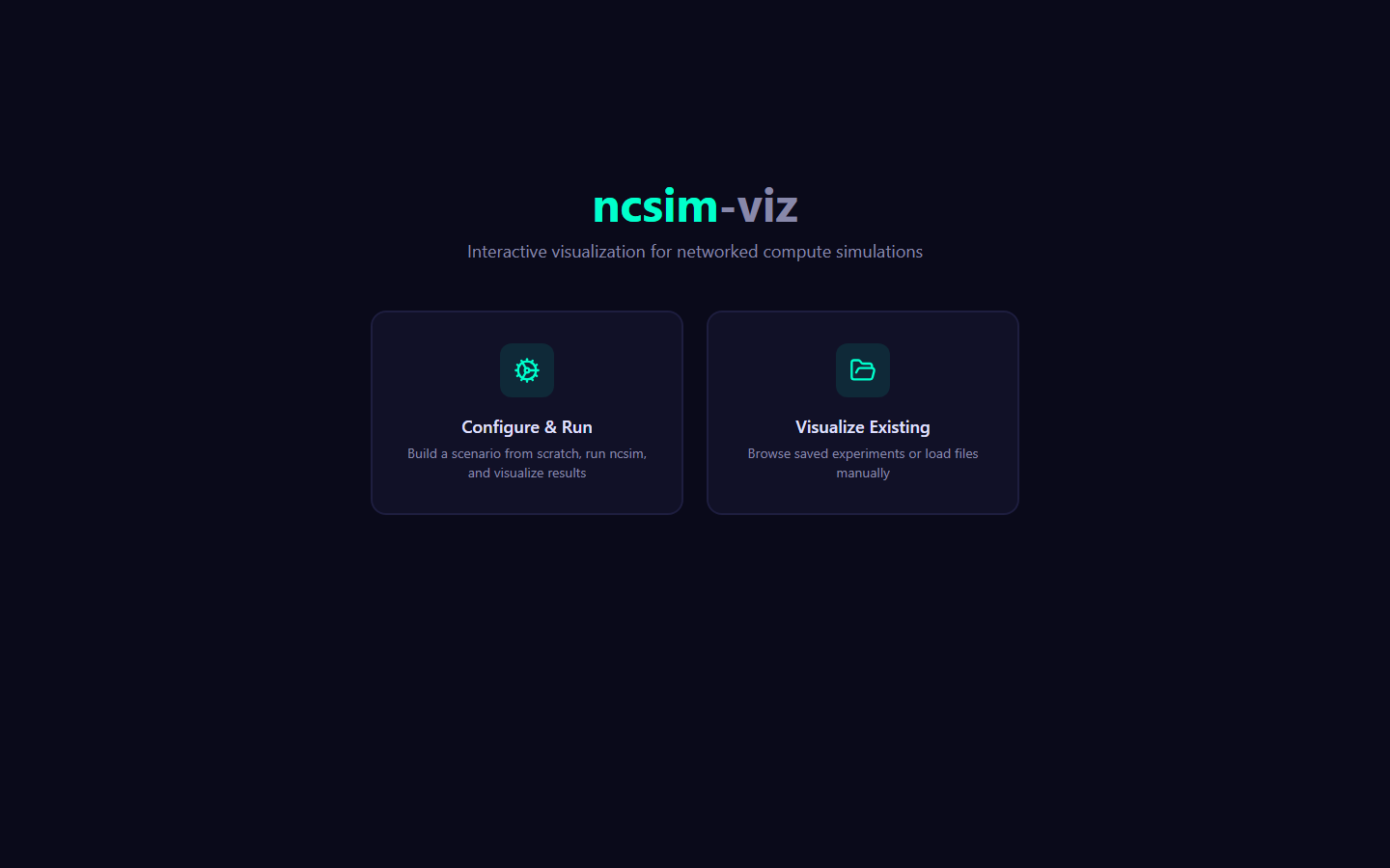
Architecture
ncsim-viz is a two-process application: a React frontend and a FastAPI backend.
| Layer | Technology | Default Port |
|---|---|---|
| Frontend | React 19 + TypeScript, Vite dev server, Tailwind CSS 4, D3.js 7 + Dagre, Lucide React icons | 5173 |
| Backend | FastAPI + uvicorn, runs ncsim via subprocess | 8000 |
The Vite development server proxies all /api/* requests to the FastAPI backend on port 8000. When the user submits a scenario, the frontend sends the generated YAML to the backend, which invokes the ncsim CLI as a subprocess and returns the scenario, trace, and metrics files to the browser.
sequenceDiagram
    participant Browser
    participant Vite as Vite (port 5173)
    participant FastAPI as FastAPI (port 8000)
    participant ncsim

    Browser->>Vite: GET /  (static assets)
    Browser->>Vite: POST /api/run {yaml}
    Vite->>FastAPI: proxy /api/run
    FastAPI->>ncsim: subprocess.run(["python", "ncsim/main.py", ...])
    ncsim-->>FastAPI: trace.jsonl, metrics.json
    FastAPI-->>Browser: {scenario_yaml, trace_jsonl, metrics_json}
Workflow Modes
ncsim-viz supports two workflow modes, accessible from the home page:
1. Configure & Run
Build a scenario interactively using the form-based editor, submit it to the backend for execution, and visualize the results immediately. This mode requires both the frontend and backend servers to be running.
2. Visualize Existing
Browse saved experiments from the sample-runs/ directory, or load your own output files (scenario YAML, trace JSONL, and metrics JSON). When browsing pre-generated sample runs, this mode can work with just the frontend server if the experiments are available as static files.
Both modes lead to the same visualization
Regardless of how data is loaded, the same six visualization tabs are available once results are present.
Visualization Tabs
After loading or running an experiment, the UI presents six tabs:
| Tab | Key | Description |
|---|---|---|
| Overview | 1 | Dashboard of key metrics: makespan, task/transfer counts, utilization bars, WiFi summary |
| Network | 2 | Interactive D3 force-directed graph of the network topology |
| DAG | 3 | Dagre hierarchical layout of the task dependency graph |
| Schedule | 4 | Static Gantt chart showing task execution and data transfers over time |
| Simulation | 5 | Animated event replay with live network overlay, growing Gantt, and event log |
| Parameters | 6 | Read-only inspector of the complete experiment configuration |
Directory Structure
viz/
├── src/                  # React frontend
│   ├── App.tsx           # Main app shell with routing
│   ├── main.tsx          # React entry point
│   ├── components/
│   │   ├── home/         # HomePage: two-column layout, ExperimentBrowser
│   │   ├── configure/    # ExperimentForm, TopologySection, DagSection,
│   │   │                 # InterferenceSection, YamlPreview
│   │   ├── layout/       # AppShell, TabBar, ThemeToggle
│   │   ├── loader/       # FileLoader: manual file upload
│   │   ├── overview/     # OverviewPanel: summary metrics and utilization
│   │   ├── network/      # NetworkView: D3 force-directed graph, NodeTooltip
│   │   ├── dag/          # DagView: Dagre hierarchical layout, TaskTooltip
│   │   ├── gantt/        # GanttChart: static and animated D3 Gantt
│   │   ├── simulation/   # SimulationView, TimelineControls, EventLog
│   │   └── parameters/   # ParametersPanel: config inspector
│   ├── hooks/            # React hooks (useSimulation, usePlayback,
│   │                     # useRunExperiment, useExperiments)
│   ├── loaders/          # YAML / JSONL / JSON parsers
│   ├── engine/           # SimulationState: animation state machine
│   ├── theme/            # Color palette utilities
│   └── types/            # TypeScript interfaces (scenario, trace, metrics, api)
├── server/               # FastAPI backend
│   ├── main.py           # API endpoints (/api/run, /api/experiments)
│   ├── run.py            # Startup script (uvicorn launcher)
│   └── requirements.txt  # Python dependencies (fastapi, uvicorn)
├── public/
│   └── sample-runs/      # Pre-generated experiment results
├── vite.config.ts        # Vite config with /api proxy to port 8000
├── package.json          # npm dependencies and scripts
└── tsconfig.json         # TypeScript configuration
API Endpoints
The FastAPI backend exposes three endpoints:
| Method | Path | Description |
|---|---|---|
GET |
/api/experiments |
List all saved experiments in sample-runs/ with summary metadata |
GET |
/api/experiments/{name} |
Load all files (scenario YAML, trace JSONL, metrics JSON) for a specific experiment |
POST |
/api/run |
Run ncsim with the provided scenario YAML and return results |
Sequential execution
The backend uses a lock to ensure only one ncsim subprocess runs at a time. Concurrent run requests will queue behind the lock. Simulations time out after 60 seconds.
Next Steps
- Viz Setup -- Install dependencies and start the servers
- Configure & Run -- Walkthrough of the experiment configuration form
- Visualization Tabs -- Detailed guide to each visualization tab
- Keyboard Shortcuts -- Full shortcut reference
Viz Setup
This page walks through installing dependencies and starting the ncsim-viz frontend and backend servers.
Prerequisites
Before setting up ncsim-viz, ensure you have:
| Requirement | Minimum Version | Check Command |
|---|---|---|
| Python | 3.10+ | python --version |
| Node.js | 18+ | node --version |
| npm | 9+ | npm --version |
| ncsim | Installed in editable mode | python -c "import ncsim" |
ncsim must be installed first
The backend invokes ncsim as a subprocess. If you have not yet installed ncsim, follow the Installation guide first:
Install Backend Dependencies
The backend requires FastAPI and uvicorn. Install them from the server requirements file:
This installs:
fastapi>=0.115.0-- the async web framework that serves the APIuvicorn>=0.34.0-- the ASGI server that runs FastAPI
Install Frontend Dependencies
Install the Node.js packages for the React frontend:
Key frontend dependencies include:
| Package | Purpose |
|---|---|
react / react-dom |
UI framework (React 19) |
d3 |
Network graph and Gantt chart rendering |
dagre |
Hierarchical DAG layout algorithm |
js-yaml |
YAML parsing for scenario preview |
lucide-react |
Icon library |
tailwindcss |
Utility-first CSS framework (v4) |
vite |
Development server and build tool |
Start the Servers
ncsim-viz requires two servers running simultaneously. Open two terminal windows:
Terminal 1 -- Backend
You should see output similar to:
INFO:     Uvicorn running on http://127.0.0.1:8000 (Press CTRL+C to quit)
INFO:     Started reloader process
The FastAPI backend is now serving on http://localhost:8000. It auto-reloads when you edit server files.
Terminal 2 -- Frontend
You should see output similar to:
The Vite development server is now serving on http://localhost:5173.
Open your browser
Navigate to http://localhost:5173 to access the ncsim-viz UI.
How the Proxy Works
The Vite configuration (viz/vite.config.ts) includes a proxy rule that forwards all /api/* requests from the frontend dev server (port 5173) to the FastAPI backend (port 8000):
This means:
- Both servers must be running for the Configure & Run workflow (which calls
POST /api/run) - Visualize Existing mode also calls
/api/experimentsto list and load saved experiments, so the backend is needed for browsing sample runs as well - The browser always connects to port 5173 -- it never talks directly to port 8000
Verify the Setup
After both servers are running, verify everything works:
-
Home page -- Open http://localhost:5173 and confirm you see the home page with two workflow cards: "Configure & Run" and "Visualize Existing".
-
Browse experiments -- Click "Visualize Existing". You should see a list of saved experiments from the
sample-runs/directory (if any exist). -
Load an experiment -- Click on any listed experiment. The Overview tab should appear, displaying metrics such as makespan, task count, and utilization bars.
-
Run an experiment -- Click "Configure & Run", leave the default settings, and click "Run Experiment". The backend should execute ncsim and display the results.
No sample runs?
If the experiment browser shows no experiments, the viz/public/sample-runs/ directory may be empty. Run a simulation first using the CLI or the Configure & Run workflow to populate it.
Production Build
To create an optimized production build of the frontend:
This runs the TypeScript compiler followed by Vite's production bundler. The output is written to the viz/dist/ directory. You can serve these static files with any web server, but you will still need the FastAPI backend running for experiment execution and browsing.
Preview the production build
After building, you can preview the production output locally:
This starts a local server serving the dist/ directory, useful for verifying the build before deployment.
Troubleshooting
| Problem | Solution |
|---|---|
ModuleNotFoundError: No module named 'ncsim' |
Install ncsim in editable mode: pip install -e . from the repo root |
ModuleNotFoundError: No module named 'fastapi' |
Run pip install -r viz/server/requirements.txt |
| Port 8000 already in use | Stop the other process, or edit viz/server/run.py to use a different port |
| Port 5173 already in use | Vite will automatically try the next available port (5174, 5175, etc.) |
| "Run Experiment" button shows error | Confirm the backend is running on port 8000 and the proxy is configured correctly |
| CORS errors in browser console | Make sure you are accessing the frontend through port 5173 (not 8000 directly) |
Next Steps
- Configure & Run -- Build and run an experiment using the form editor
- Visualization Tabs -- Explore the six visualization views
Configure & Run
The Configure & Run workflow lets you build a scenario interactively, submit it to the backend, and visualize results immediately. This page provides a full walkthrough of the configuration form.
Basic Configuration
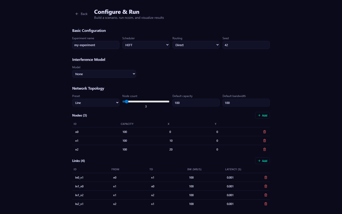
The top section of the form contains four fields that control the core simulation parameters.
| Field | Type | Default | Description |
|---|---|---|---|
| Experiment name | text | my-experiment |
Identifies this run. Used as the directory name for saved results. |
| Scheduler | select | heft |
Task scheduling algorithm. See options below. |
| Routing | select | direct |
Routing mode for data transfers between nodes. |
| Seed | number | 42 |
Random seed for deterministic reproducibility. |
Scheduler Options
| Value | Algorithm | Description |
|---|---|---|
heft |
HEFT | Heterogeneous Earliest Finish Time -- prioritizes tasks by upward rank, assigns each to the node that gives the earliest finish |
cpop |
CPOP | Critical Path on a Processor -- identifies the critical path and schedules critical tasks on the fastest processor |
round_robin |
Round Robin | Assigns tasks to nodes in a round-robin rotation |
manual |
Manual | You assign each task to a specific node using the "Pinned To" column in the DAG section |
Routing Options
| Value | Algorithm | Description |
|---|---|---|
direct |
Direct | Uses only explicitly declared links (single-hop). Fails if no direct link exists. |
widest_path |
Widest Path | Finds the multi-hop path that maximizes bottleneck bandwidth. |
shortest_path |
Shortest Path | Finds the multi-hop path that minimizes total latency (hop count). |
Manual scheduler
When you select the manual scheduler, the "Pinned To" column in the DAG Structure section switches from a free-text input to a dropdown populated with all defined node IDs, making it easy to assign each task to a specific node.
Interference Model
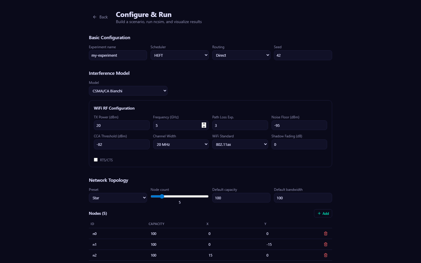
The Interference Model section lets you select how concurrent wireless transmissions affect each other. The form dynamically shows or hides fields based on your selection.
Available Models
| Model | Behavior | Extra Fields Shown |
|---|---|---|
| None | No interference. Links use their declared bandwidth at all times. | -- |
| Proximity | Links within a configurable radius of each other share bandwidth. | Radius (m) |
| CSMA/CA Clique | Static clique-based model. Link bandwidth = PHY rate / max clique size. | WiFi RF Configuration panel |
| CSMA/CA Bianchi | Bianchi saturation throughput model. MAC throughput derived from collision probability and backoff parameters. | WiFi RF Configuration panel |
WiFi RF Configuration
When you select either CSMA/CA model, a dedicated panel appears with the following PHY-layer parameters:
| Field | Default | Description |
|---|---|---|
| TX Power (dBm) | 20 | Transmit power |
| Frequency (GHz) | 5.0 | Carrier frequency |
| Path Loss Exponent | 3.0 | Log-distance path loss exponent |
| Noise Floor (dBm) | -95 | Receiver noise floor |
| CCA Threshold (dBm) | -82 | Clear Channel Assessment threshold |
| Channel Width | 20 MHz | Channel bandwidth (20, 40, 80, or 160 MHz) |
| WiFi Standard | 802.11ax | Standard for MCS rate table (802.11n, 802.11ac, or 802.11ax) |
| Shadow Fading (dB) | 0 | Standard deviation of log-normal shadow fading |
| RTS/CTS | Off | Enable Request-to-Send / Clear-to-Send handshake |
RF parameters affect topology generation
When the topology preset is set to "Random (radio-range)", the RF parameters (TX power, frequency, path loss exponent, noise floor) determine the radio range. Links are automatically generated between nodes that fall within this computed range. Changing RF parameters will regenerate the random topology.
Network Topology
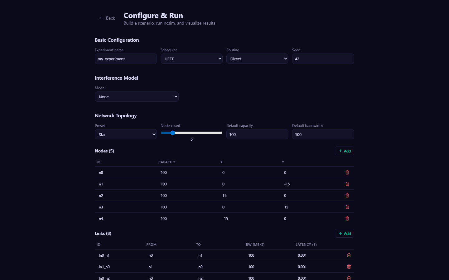
The Network Topology section defines the compute nodes and communication links of the network.
Topology Presets
Select a preset to auto-generate a topology, or choose Custom to define nodes and links manually.
| Preset | Shape | Link Pattern |
|---|---|---|
| Line | Chain | n-1 sequential links connecting nodes in order |
| Ring | Closed loop | n links forming a cycle |
| Star | Hub-and-spoke | n-1 links from a central hub to all other nodes |
| Mesh (fully connected) | Complete graph | n(n-1)/2 links connecting every pair of nodes |
| Grid | 2D grid | Horizontal and vertical links in a grid pattern |
| Random (radio-range) | Position-based | Links created between nodes within the computed radio range |
| Custom | Manual | No auto-generation; define nodes and links by hand |
Topology Parameters
| Parameter | Range | Description |
|---|---|---|
| Node count | 2 -- 20 | Number of compute nodes (slider) |
| Default capacity | 1+ | Default compute capacity (CU/s) for generated nodes |
| Default bandwidth | 0.1+ | Default bandwidth (MB/s) for generated links |
Nodes Table
Each node has the following editable fields:
| Column | Description |
|---|---|
| ID | Unique node identifier (e.g., n0, n1) |
| Capacity | Compute capacity in CU/s |
| X | X-coordinate position |
| Y | Y-coordinate position |
You can add nodes with the Add button or remove individual nodes with the trash icon. When using a preset other than Custom, editing the table switches the mode to Custom.
Links Table
Each link has the following editable fields:
| Column | Description |
|---|---|
| ID | Unique link identifier (e.g., l0, l1) |
| From | Source node ID |
| To | Target node ID |
| BW (MB/s) | Bandwidth in megabytes per second |
| Latency (s) | Propagation latency in seconds |
DAG Structure
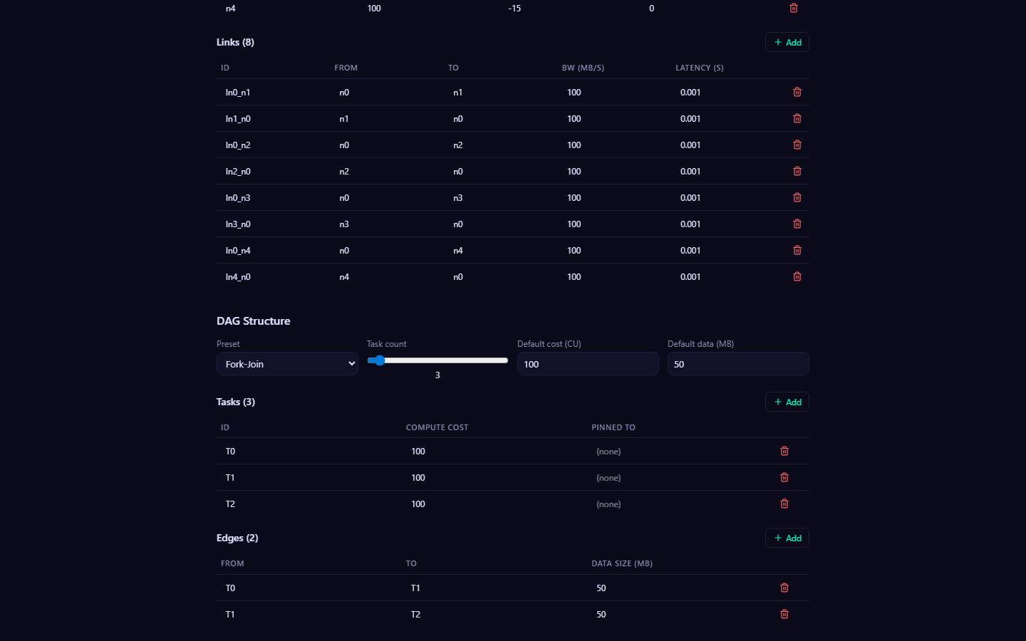
The DAG Structure section defines the task dependency graph that the scheduler will map onto the network.
DAG Presets
| Preset | Shape | Description |
|---|---|---|
| Chain | Sequential | Each task depends on the previous one, forming a linear chain |
| Fork-Join | Fan-out / fan-in | A root task fans out to parallel workers, which all converge to a sink task |
| Diamond | Two-level | Root fans to parallel middle layer, which merges, then fans again to a second layer before the final sink |
| Parallel (independent) | Independent | All tasks are independent with no data dependencies |
| Custom | Manual | No auto-generation; define tasks and edges by hand |
DAG Parameters
| Parameter | Range | Description |
|---|---|---|
| Task count | 2 -- 20 | Number of tasks (slider) |
| Default cost (CU) | 1+ | Default compute cost in compute units for generated tasks |
| Default data (MB) | 0.1+ | Default data size in megabytes for generated edges |
Tasks Table
| Column | Description |
|---|---|
| ID | Unique task identifier (e.g., T0, T1) |
| Compute Cost | Compute cost in CU (compute units) |
| Pinned To | Optional: force this task onto a specific node (used with manual scheduler, or to override any scheduler) |
Edges Table
| Column | Description |
|---|---|
| From | Source task ID (producer) |
| To | Target task ID (consumer) |
| Data Size (MB) | Volume of data transferred between tasks |
YAML Preview
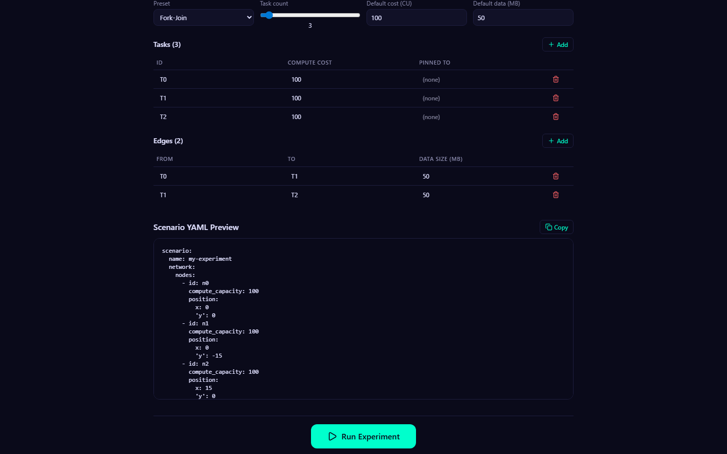
At the bottom of the form, a live YAML preview shows the complete scenario definition that will be sent to the backend. This YAML updates in real time as you modify any form field.
The preview includes:
- Scenario name
- Full network definition (nodes with positions and capacities, links with bandwidths and latencies)
- DAG definition (tasks with compute costs, edges with data sizes)
- Config section (scheduler, seed, routing, interference model, and RF parameters if applicable)
Reusable scenarios
Click the Copy button to copy the YAML to your clipboard. You can save it as a .yaml file and reuse it with the ncsim CLI:
Running the Experiment
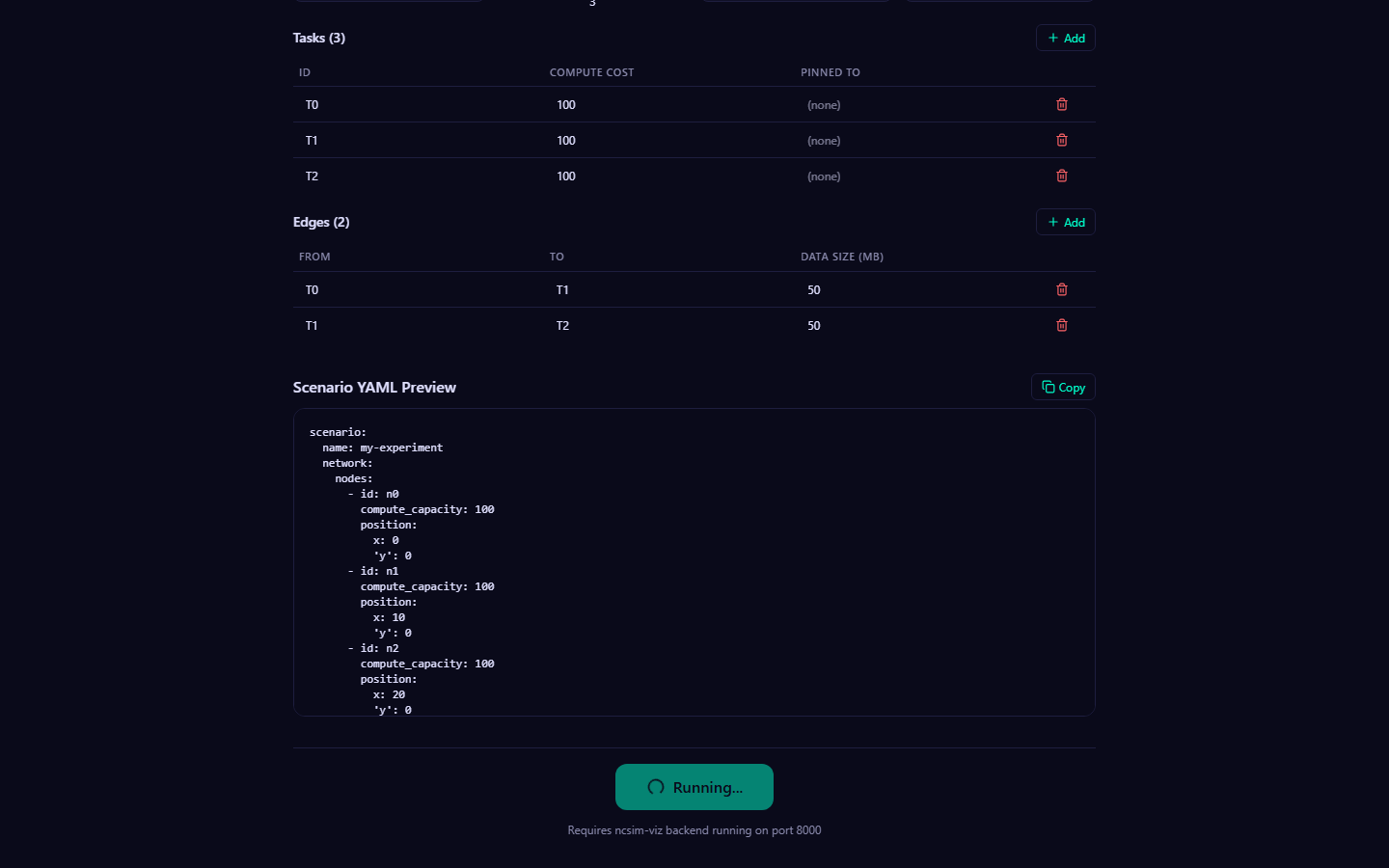
Click the Run Experiment button at the bottom of the form to submit the scenario to the backend.
The backend performs the following steps:
- Writes the scenario YAML to a temporary directory
- Invokes ncsim as a subprocess with
--scenarioand--outputflags - Reads the generated
trace.jsonlandmetrics.jsonfiles - Returns all three files (scenario YAML, trace JSONL, metrics JSON) to the frontend
- Saves the results in
viz/public/sample-runs/for future browsing
Execution time
Simple scenarios (a few nodes and tasks, no interference) complete in under 2 seconds. Complex WiFi scenarios with CSMA/CA Bianchi interference may take longer. The backend enforces a 60-second timeout.
After the run completes successfully, the UI automatically transitions to the visualization view, starting on the Overview tab. If the run fails, an error message is displayed below the Run button with details from ncsim's stderr output.
Backend required
The Run Experiment button requires the FastAPI backend to be running on port 8000. If the backend is not available, the button will show an error. See Viz Setup for instructions on starting both servers.
Next Steps
- Visualization Tabs -- Explore the results across all six tabs
- Keyboard Shortcuts -- Navigate the UI efficiently
Visualization Tabs
After running an experiment or loading saved results, ncsim-viz presents six visualization tabs. Switch between them by clicking the tab bar or pressing number keys 1 through 6.
Overview Tab
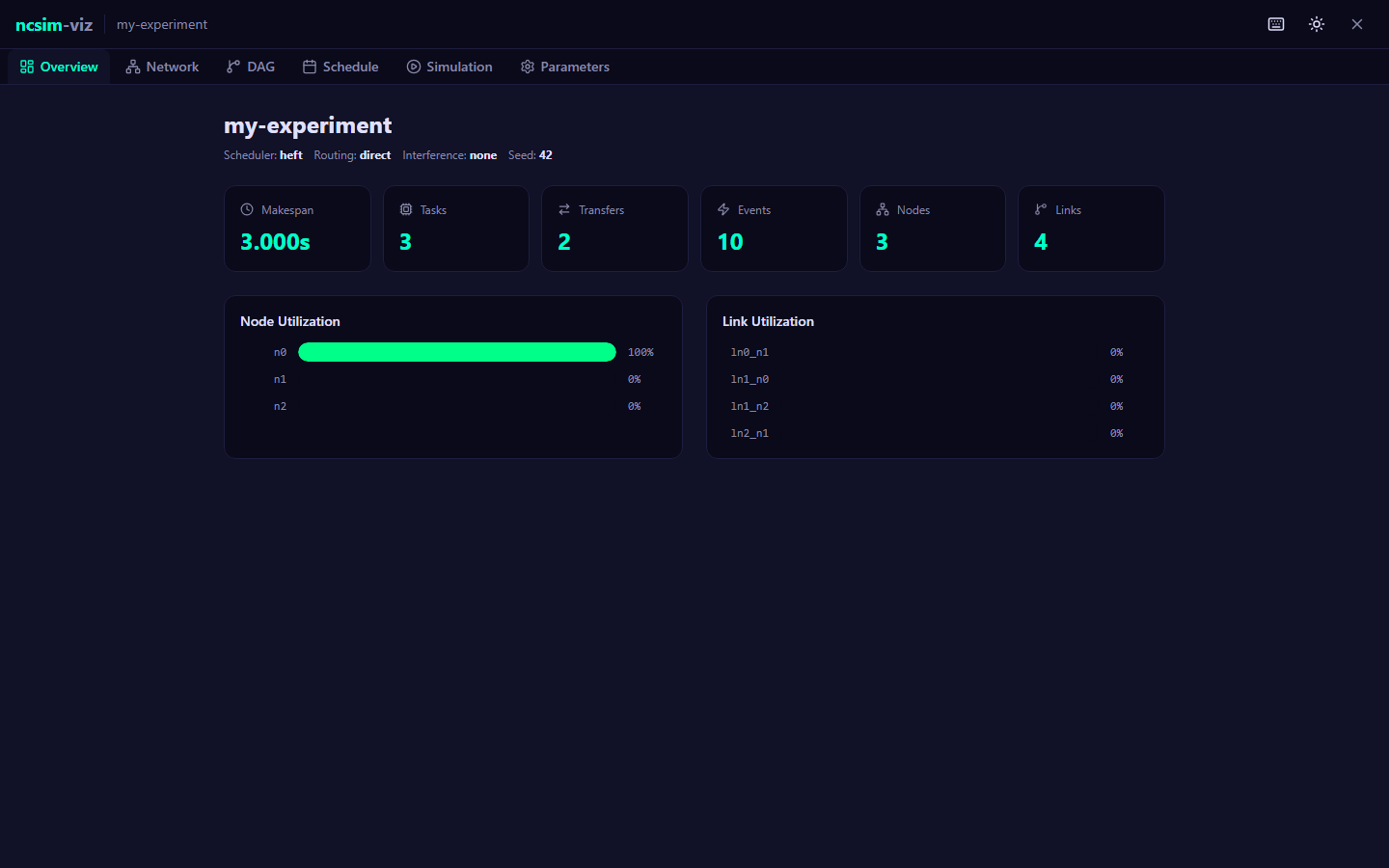
The Overview tab provides a high-level dashboard of the experiment results.
Header
Displays the scenario name along with key configuration metadata: scheduler algorithm, routing mode, interference model, and random seed.
Metric Cards
Six summary cards are shown in a grid:
| Metric | Description |
|---|---|
| Makespan | Total simulation time from first event to last (seconds) |
| Tasks | Total number of tasks executed |
| Transfers | Total number of data transfers between nodes |
| Events | Total number of discrete events in the trace |
| Nodes | Number of compute nodes in the network |
| Links | Number of communication links in the network |
Utilization Charts
Two side-by-side panels display per-resource utilization as horizontal bar charts:
- Node Utilization -- Percentage of the makespan each node spent executing tasks. Color varies by utilization level: accent color for moderate utilization (>30%), green for high utilization (>70%).
- Link Utilization -- Percentage of the makespan each link spent transferring data. If all tasks were assigned to the same node (no remote transfers), this panel shows a "No link utilization data" message.
WiFi Configuration Summary
When a CSMA interference model was used, an additional panel displays the RF configuration parameters (TX power, frequency, path loss exponent, etc.) and the computed carrier sensing range.
Network Tab
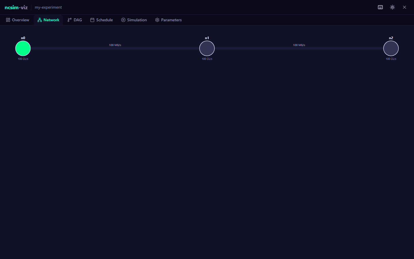
The Network tab renders an interactive D3-based visualization of the network topology.
Node Rendering
- Nodes are drawn as circles sized proportional to compute capacity -- higher capacity nodes appear larger
- Node color reflects utilization: green for high utilization (>50%), themed color for moderate utilization (>10%), gray for low/unused nodes
- Each node is labeled with its ID above the circle and its capacity (CU/s) below
Link Rendering
- Links are drawn as lines connecting their endpoint nodes
- Line thickness is proportional to bandwidth -- wider lines indicate higher bandwidth links
- Each link is labeled at its midpoint with the bandwidth value (MB/s)
Interactions
| Action | Effect |
|---|---|
| Drag background | Pan the view |
| Scroll wheel | Zoom in/out (0.3x to 5x) |
| Hover over node | Shows tooltip with node ID, compute capacity, and utilization percentage |
Responsive layout
The network graph automatically rescales when the browser window is resized. Node positions are computed from the position coordinates in the scenario YAML, mapped to screen space with padding.
DAG Tab
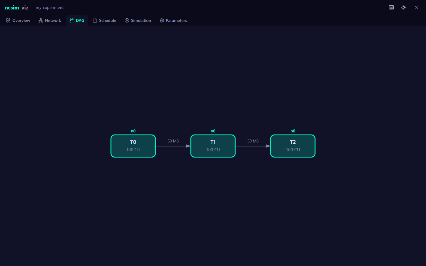
The DAG tab shows the task dependency graph using a Dagre hierarchical layout with left-to-right flow direction.
Task Nodes
- Each task is drawn as a rounded rectangle with the task ID and compute cost (CU)
- Tasks are colored by their assigned compute node -- tasks assigned to the same node share the same color, making it easy to see the scheduler's placement decisions
- A small badge above each task node shows the assigned node ID
- Unassigned tasks appear in gray
Edges
- Edges represent data dependencies between tasks
- Edge labels show the data transfer size in MB
- Edges are drawn as curved spline paths with arrowheads indicating direction
Interactions
| Action | Effect |
|---|---|
| Drag background | Pan the view |
| Scroll wheel | Zoom in/out (0.3x to 3x) |
| Hover over task | Shows tooltip with task ID, compute cost, assigned node, start time, and end time |
Schedule Tab
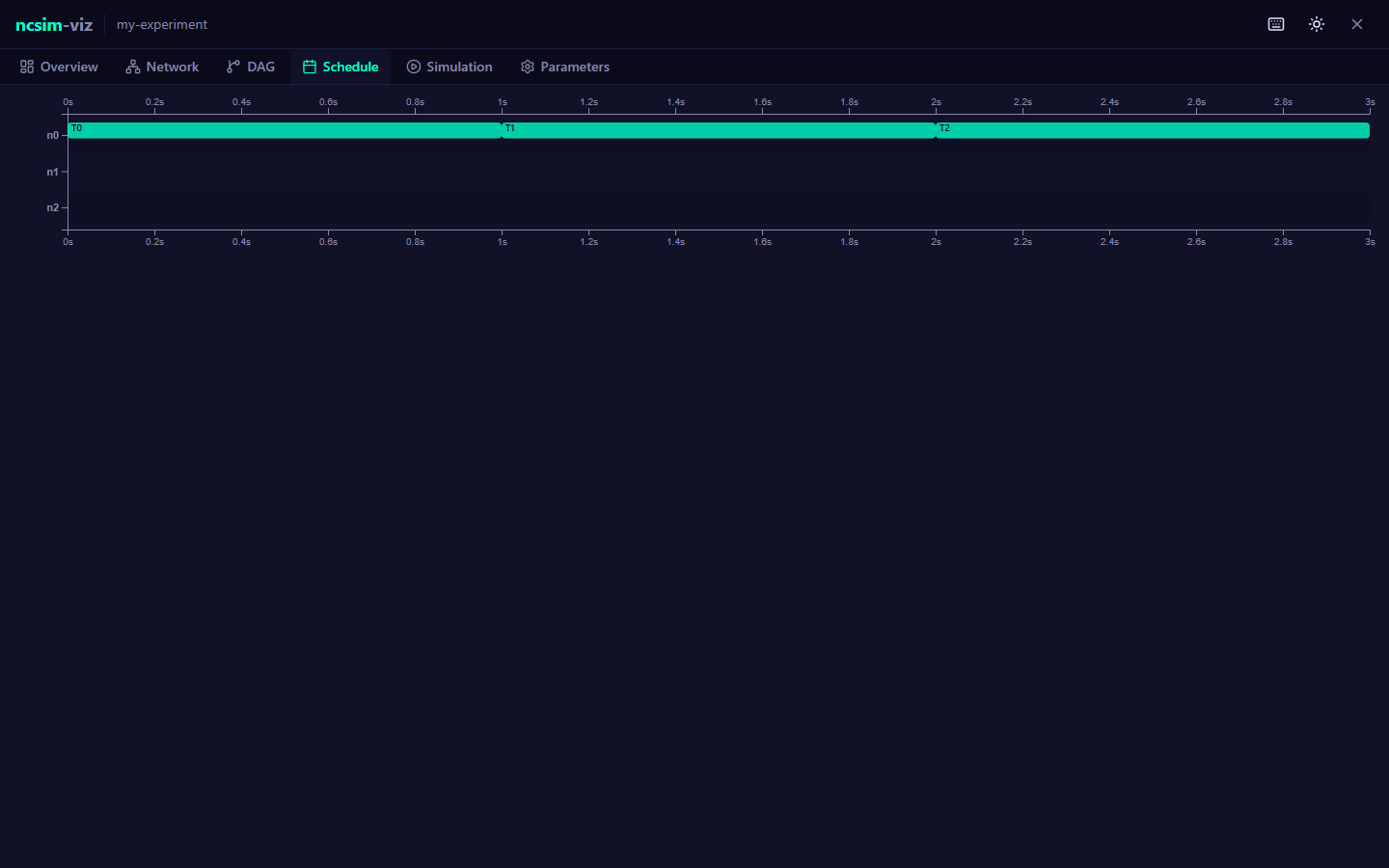
The Schedule tab presents a static Gantt chart of the full simulation timeline.
Axes
- X-axis (top and bottom): Simulation time in seconds, from 0 to the makespan
- Y-axis: Compute nodes, one row per node
Task Bars
- Colored rectangles spanning each task's execution period on its assigned node
- Color matches the node's color scheme for consistency with other views
- Task IDs are displayed inside bars when there is sufficient width
- Hover over a task bar for a tooltip showing: task ID, node ID, start time, end time, and duration
Transfer Bars
- Hatched (dashed-outline) rectangles below the task bars, representing data transfers
- Positioned on the source node's row
- Colored in magenta to visually distinguish transfers from compute tasks
- Hover over a transfer bar for a tooltip showing: source task, destination task, link ID, data size, start time, and end time
Alternating Rows
Every other node row has a subtle background tint to improve readability when many nodes are present.
Simulation Tab
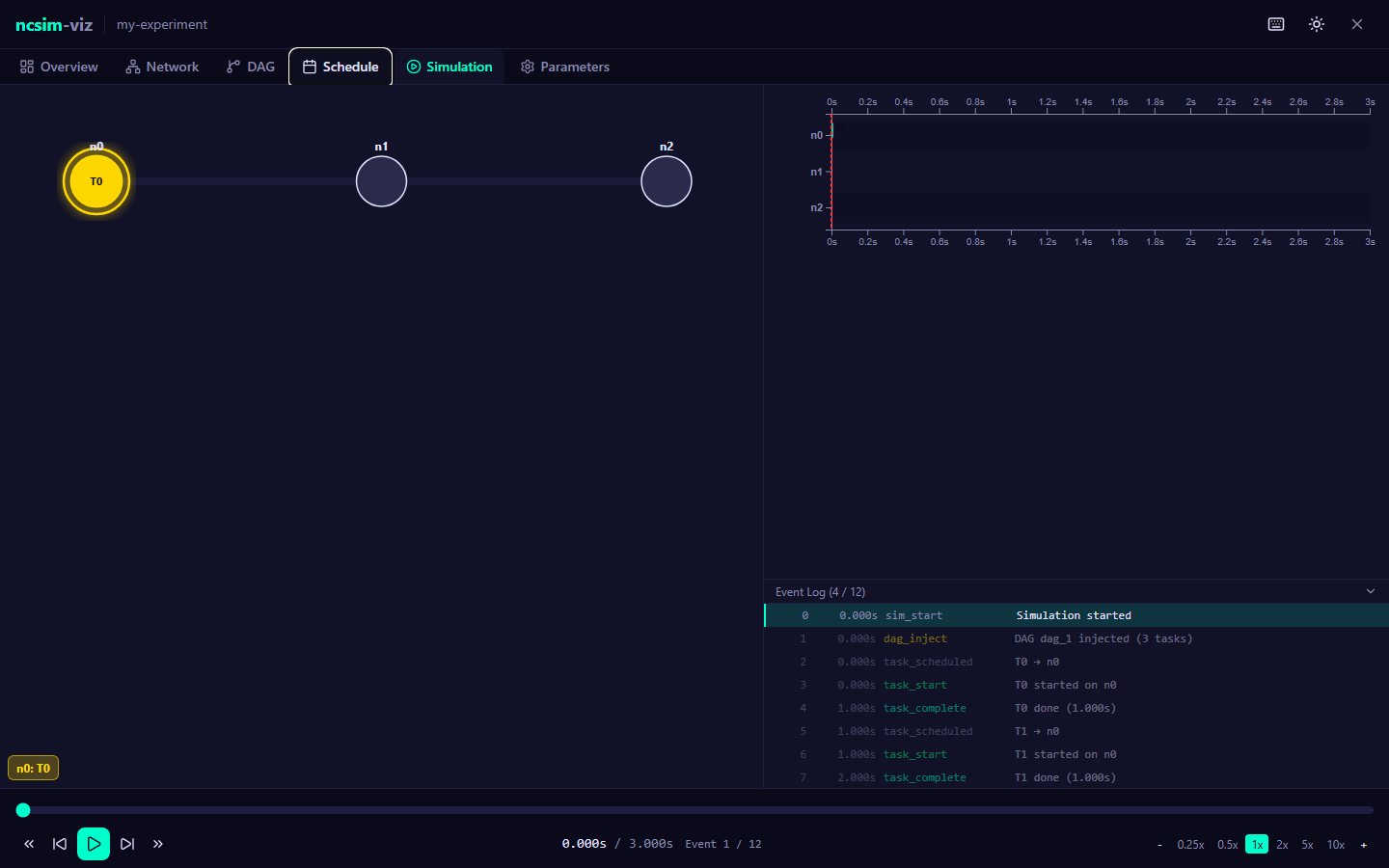
The Simulation tab provides an animated event-by-event replay of the simulation, combining multiple synchronized views.
Layout
The simulation view is split into three coordinated panels:
| Panel | Position | Content |
|---|---|---|
| Network overlay | Left (55% width) | Animated network graph with active-state highlighting |
| Live Gantt chart | Right top | Gantt chart that grows as the simulation progresses |
| Event log | Right bottom (collapsible) | Scrolling list of all trace events |
Network Animation
During playback, the network graph shows real-time state changes:
- Active nodes (currently executing a task): highlighted in gold with a pulsing ring animation, with the current task name displayed inside the node circle
- Completed nodes (finished at least one task): shown in green with a checkmark and completed task count
- Idle nodes: shown in dim gray
- Active links (currently transferring data): shown in magenta with animated dashed lines and a glow effect, with the transfer label (source task to destination task) displayed at the link midpoint
- Inactive links: shown as faint lines
Live Gantt Chart
The Gantt chart in the Simulation tab is time-synchronized with the playback:
- Task and transfer bars grow in real time as the simulation progresses
- A red vertical playhead line tracks the current simulation time
- Only events that have occurred up to the current time are visible
Event Log
A scrolling log at the bottom-right displays every trace event:
| Column | Content |
|---|---|
| Sequence number | Event ordering index |
| Time | Simulation timestamp (seconds) |
| Type | Event type (e.g., task_start, transfer_complete) |
| Summary | Human-readable description of the event |
Events are color-coded by type:
- Green for
task_start - Accent color for
task_complete - Magenta for transfer events
- Yellow for
dag_inject
The currently active event is highlighted with a left border. Click any event to jump the playback to that point in time. Future events (beyond the current playback time) appear dimmed.
Collapsible log
Click the "Event Log" header to collapse or expand the event log panel, giving more vertical space to the Gantt chart.
Playback Controls
The transport bar at the bottom provides full playback control:
| Control | Description |
|---|---|
| Scrubber | Drag the slider to seek to any point in the simulation |
| Play / Pause | Toggle playback (also via Space key) |
| Step backward / forward | Move to the previous or next event |
| Jump to start / end | Jump to time 0 or the makespan |
| Speed buttons | Select playback speed: 0.25x, 0.5x, 1x, 2x, 5x, or 10x |
| +/- buttons | Increment or decrement speed one step |
The time display shows the current time, total makespan, and current event index out of total events.
Parameters Tab
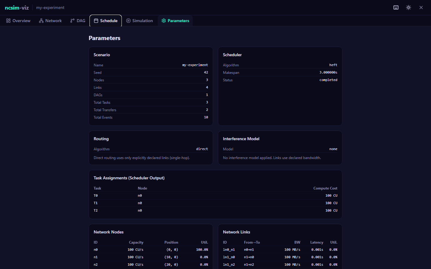
The Parameters tab is a read-only inspector that displays the complete configuration and results of the experiment.
Sections
The parameters are organized into collapsible sections:
- Scenario
-
Experiment name, seed, node count, link count, DAG count, total tasks, total transfers, total events.
- Scheduler
-
Algorithm name, computed makespan, simulation completion status.
- Routing
-
Algorithm name with a brief description of its behavior.
- Interference Model
-
Selected model name, radius (if proximity), and a description of the model's behavior.
- WiFi RF Configuration (shown only when CSMA model was used)
-
All PHY parameters: TX power, frequency, path loss exponent, noise floor, CCA threshold, channel width, WiFi standard, shadow fading sigma, RTS/CTS.
- Derived WiFi Values (shown only when CSMA model was used)
-
Carrier sensing range, per-link PHY rates (MB/s), and max clique sizes.
- Task Assignments
-
Table showing the scheduler's output: each task ID, its assigned node, and compute cost.
- Network Nodes
-
Table with each node's ID, compute capacity, position coordinates, and utilization percentage.
- Network Links
-
Table with each link's ID, endpoints, bandwidth, latency, and utilization percentage.
- DAG Edges
-
Table with each data dependency's source task, destination task, and data size.
Next Steps
- Keyboard Shortcuts -- Full reference for navigating the UI with the keyboard
- Configure & Run -- Build a new experiment using the form editor
Keyboard Shortcuts
ncsim-viz supports keyboard shortcuts for efficient navigation and playback control. Press ? at any time to display the shortcut overlay within the application.
Full Reference
| Key | Action |
|---|---|
| Space | Play / Pause simulation |
| Left | Step backward one event |
| Right | Step forward one event |
| Shift+Left | Jump backward 10% of the makespan |
| Shift+Right | Jump forward 10% of the makespan |
| Home | Jump to the start of the simulation (time 0) |
| End | Jump to the end of the simulation (makespan) |
| + | Increase playback speed one step |
| - | Decrease playback speed one step |
| 1 | Switch to the Overview tab |
| 2 | Switch to the Network tab |
| 3 | Switch to the DAG tab |
| 4 | Switch to the Schedule tab |
| 5 | Switch to the Simulation tab |
| 6 | Switch to the Parameters tab |
| D | Toggle dark / light theme |
| ? | Show / hide keyboard shortcuts overlay |
Playback Speed Levels
The + and - keys cycle through the following speed values:
| Level | Speed |
|---|---|
| 1 | 0.25x |
| 2 | 0.5x |
| 3 | 1x (default) |
| 4 | 2x |
| 5 | 5x |
| 6 | 10x |
You can also click the speed buttons in the transport bar on the Simulation tab to jump directly to any speed level.
Scope and Behavior
Shortcuts work on all tabs
Tab switching (1 through 6) and the theme toggle (D) work from any visualization tab, not just the Simulation tab. Playback controls (Space, arrow keys, Home/End, +/-) are active whenever the Simulation tab's playback engine is loaded.
Text input fields
Keyboard shortcuts are automatically disabled when focus is inside a text input field or text area, so you can type normally in the Configure & Run form without triggering shortcuts.
Shortcut Overlay
Press ? to open the shortcuts overlay. The overlay displays all shortcuts in a modal dialog. Press ? again or click outside the modal to dismiss it. You can also open the overlay by clicking the keyboard icon in the header toolbar.
Related Pages
- Visualization Tabs -- Detailed guide to each tab and its interactive features
- Viz Overview -- Architecture and workflow overview
Experiments
Interference Verification
The run_interference_verification.py script validates the csma_bianchi WiFi
interference model by comparing simulation results against analytical predictions
computed directly from the WiFi RF functions. It runs nine experiments
covering single-link PHY rates, parallel-link contention, hidden terminal SINR
degradation, multi-phase rate transitions, bandwidth sharing, and combined
effects.
Running the Script
Output directory: /tmp/ncsim_interference_verification (configurable via the
OUTDIR variable in the script).
Default RF Configuration
All experiments use the same default RFConfig:
| Parameter | Value |
|---|---|
| TX power | 20 dBm |
| Frequency | 5 GHz |
| Path loss exponent | 3.0 |
| Noise floor | -95 dBm |
| CCA threshold | -82 dBm |
| Channel width | 20 MHz |
| WiFi standard | 802.11ax |
| Shadow fading | 0 (disabled) |
| RTS/CTS | disabled |
Data size per transfer: 10 MB. Tolerance for all checks: 1%.
Experiment 1: Link Length vs Data Rate (Single Link)
Varies the distance between a single transmitter-receiver pair (n0 to n1)
with no other links present.
- Purpose: Verify that the PHY rate matches the analytical SNR-to-MCS prediction when there is zero interference.
- Distances tested: 1m, 3m, 5m, 8m, 12m, 16m, 20m, 25m, 30m, 36m, 42m, 50m, 58m, 66m, 75m, 85m, 95m, 105m, 120m, 140m.
- Analytical prediction:
rate_mbps_to_MBps(snr_to_rate_mbps(snr_dB(received_power_dBm(tx, d, rf), noise))) - Verification: Simulated data rate (computed as
data_size / duration) matches the predicted rate within 1%.
At distances beyond the minimum MCS threshold (SNR < 5 dB), the PHY rate drops to zero and the simulator uses a 0.001 MB/s fallback.
Experiment 2: Parallel Link Separation vs Interference
Two parallel 30m horizontal links separated by a variable vertical distance.
- Purpose: Test both contention (within carrier sensing range) and hidden terminal (outside carrier sensing range) effects.
- Separations tested: 5m, 10m, 15m, 20m, 30m, 40m, 50m, 60m, 65m, 70m, 75m, 80m, 100m, 140m, 200m.
Key Behaviors
| Regime | Condition | Behavior |
|---|---|---|
| Contention | Separation <= carrier sensing range | Both links in conflict graph. Share airtime via Bianchi MAC: each gets base_rate * eta(2) / 2. |
| Hidden terminal | Separation > carrier sensing range | Links outside conflict graph. Transmit simultaneously, causing SINR degradation at receivers. |
| No interference | Separation very large | Interferer power negligible. Both links approach solo PHY rate. |
- Verification: Both links' effective rates match analytical predictions (Bianchi contention factor for in-conflict, SINR-based rate for hidden terminal) within 1%.
Symmetry
By construction, both links in this experiment always see identical interference geometry. The script verifies that both links produce the same rate.
Experiment 3: Two Transmitters to Same Receiver
Two transmitting nodes send to a shared receiver at the origin, with transmitters placed at 90 degrees apart at equal distance.
- Purpose: Test SINR calculation when multiple transmitters target the same receiver.
- Distances tested: 5m to 130m.
- Key insight: When both links are in the conflict graph, they share airtime
via Bianchi. When they are hidden terminals, both transmitters cause
equal-power interference at the shared receiver, resulting in very low SINR
(the model clamps the interference factor to
MIN_FACTOR). - Verification: Both links' rates match predictions within 1%.
Experiment 4: Three Parallel Links
Three parallel 30m links stacked vertically at equal spacing.
Link A: n0(0, 0)     -----> n1(30, 0)
Link B: n2(0, sep)   -----> n3(30, sep)
Link C: n4(0, 2*sep) -----> n5(30, 2*sep)
- Purpose: Validate multi-interferer SINR, combined Bianchi + SINR factors, and symmetry between outer links A and C.
- Separations tested: 10m, 20m, 35m, 40m, 50m, 60m, 70m, 75m, 80m, 100m, 150m.
Three Regimes
| Regime | Condition | Description |
|---|---|---|
all_conf |
All three pairs in conflict graph | 3-way Bianchi contention. All links get base_rate * eta(3) / 3. |
mixed |
AB and BC in conflict, but AC not | Center link B contends with both; outer links A and C also see each other as hidden terminals. Multi-phase completion. |
all_hid |
No conflict graph edges | All interference is SINR-based. Multiple interferers with different distances. Multi-phase completion as links finish. |
- Verification: Predicted multi-phase effective rates match simulation within 1%. Outer links A and C always have symmetric (equal) rates.
Experiment 5: Staggered Transfer Start
Two parallel 30m links at 100m separation (hidden terminals), with Transfer A starting later than Transfer B due to a high compute cost on T0.
- Purpose: Test dynamic recalculation of SINR when transfers start and complete at different times.
- Key phases:
- Phase 1: B transmits solo at base rate for
deltaseconds. - Phase 2: Both A and B active; both degrade to SINR rate.
- Phase 3: After B completes, A returns to solo base rate.
- Phase 1: B transmits solo at base rate for
- Delay costs tested: 10000, 30000, 50000, 80000 (producing different stagger durations).
- Verification: Both transfer durations match the multi-phase analytical prediction within 1%. A and B always have equal total durations (by symmetry of phases).
Experiment 6: Per-Link Bandwidth Sharing
Multiple flows with different data sizes share a single 30m link (l01).
- Purpose: Verify that concurrent flows on the same link fairly share bandwidth, and that when faster flows complete, remaining flows see increased bandwidth (multi-phase fair sharing).
- Test cases:
- 3-flow: data sizes 5, 10, 15 MB
- 3-flow-eq: data sizes 5, 5, 15 MB (two finish simultaneously)
- 4-flow: data sizes 3, 6, 9, 12 MB
- Verification: Each flow's duration matches the multi-phase prediction from
predict_fair_share_durations()within 1%.
Experiment 7: N-Way Bianchi Scaling
N parallel 30m links at 5m vertical separation (all within carrier sensing range, forming a complete conflict graph).
- Purpose: Verify that Bianchi efficiency scales correctly from N=2 through N=8 contending stations.
- Analytical prediction: Each link gets
base_rate * eta(N) / N. - Verification: All N links have the same rate, matching the Bianchi prediction within 1%.
| N | eta(N) | Per-link share: eta(N)/N |
|---|---|---|
| 2 | ~0.94 | ~0.47 |
| 3 | ~0.88 | ~0.29 |
| 4 | ~0.82 | ~0.21 |
| 5 | ~0.77 | ~0.15 |
| 8 | ~0.65 | ~0.08 |
Experiment 8: Five-Link Hidden Terminal Cascade
Five parallel 30m links at 100m vertical separation (all hidden terminals to each other) with data sizes 2, 4, 6, 8, and 10 MB.
- Purpose: Test
data_remainingtracking through 4+ recalculation phases, SINR recomputation with a shrinking active link set, and correct completion ordering with asymmetric geometry (links at different vertical positions see different aggregate interference). - Verification: Each link's total duration matches the cascading multi-phase
prediction from
predict_hidden_cascade_durations()within 1%.
Experiment 9: Combined Bandwidth Sharing + Hidden Terminal Interference
Two flows share link l01 while a third flow on link l23 (100m away) acts as
a hidden terminal.
- Purpose: Test the interaction between per-link fair sharing and inter-link SINR interference, including multi-phase transitions as flows complete.
- Test cases:
case1: l01 flows 5/10 MB, l23 flow 8 MBcase2: l01 flows 5/10 MB, l23 flow 3 MB (l23 finishes earliest)case3: l01 flows 3/15 MB, l23 flow 20 MB (l01 flow finishes first)
- Verification: All three flow durations match the multi-phase analytical prediction within 1%.
Tolerance
All experiments use a 1% tolerance for matching simulation output to analytical predictions. The comparison functions are:
rates_match(sim, pred)-- checks|sim - pred| / pred <= 0.01durations_match(sim, pred)-- same relative tolerance on transfer durations
Interpreting Results
Each experiment prints a detailed comparison table with predicted vs. actual
values and a per-row OK / FAIL indicator.
| Result | Meaning |
|---|---|
| PASS | All rows in the experiment match within tolerance. The interference model implementation is correct for this scenario class. |
| FAIL | At least one row does not match. Indicates a bug in the interference model, SINR calculation, Bianchi efficiency, or multi-phase rate tracking. |
The final summary at the end of the script reports the pass/fail status for all nine experiments:
  Summary
  ============================
  Experiment 1 (Link Length vs Rate):            PASS
  Experiment 2 (Parallel Link Separation):       PASS
  Experiment 3 (Two TX to Same RX):              PASS
  Experiment 4 (Three Parallel Links):           PASS
  Experiment 5 (Staggered Transfer Start):       PASS
  Experiment 6 (Per-Link Bandwidth Sharing):     PASS
  Experiment 7 (N-Way Bianchi Scaling):          PASS
  Experiment 8 (Five-Link Hidden Cascade):       PASS
  Experiment 9 (Combined Sharing+Interference):  PASS

  Overall: ALL PASS
If any experiment fails
A failure indicates a regression in the interference model. Check the
printed comparison table to identify which specific distance or separation
value failed, then investigate the corresponding analytical helper and the
csma_bianchi implementation in ncsim/models/interference.py and
ncsim/models/wifi.py.
Key Imports
The script imports the following from ncsim.models.wifi for analytical
predictions:
from ncsim.models.wifi import (
    RFConfig,
    received_power_dBm,
    snr_dB,
    sinr_dB,
    snr_to_rate_mbps,
    rate_mbps_to_MBps,
    carrier_sensing_range,
    bianchi_efficiency,
    path_loss_dB,
    MCS_TABLE_AX,
)
| Function | Purpose |
|---|---|
RFConfig |
Dataclass holding all RF parameters (TX power, frequency, path loss exponent, etc.) |
received_power_dBm |
Compute received power at a given distance: P_tx - PL(d) |
snr_dB |
Signal-to-noise ratio: P_rx - noise_floor |
sinr_dB |
Signal-to-interference-plus-noise ratio (linear domain aggregation) |
snr_to_rate_mbps |
MCS table lookup: highest rate whose minimum SNR requirement is met |
rate_mbps_to_MBps |
Unit conversion from Mbps to MB/s (ncsim's internal unit) |
carrier_sensing_range |
Maximum distance at which CCA detects a transmission |
bianchi_efficiency |
Bianchi MAC saturation throughput efficiency for N contending stations |
path_loss_dB |
Log-distance path loss model |
MCS_TABLE_AX |
802.11ax MCS rate table (min_snr, rate_mbps) pairs |
Routing Comparison
The run_routing_comparison.py script compares widest_path vs
shortest_path routing under HEFT scheduling with csma_bianchi WiFi
interference. It runs 18 simulations across a grid of network sizes, DAG sizes,
and routing strategies, then prints detailed comparison tables.
Running the Script
Output directory: /tmp/ncsim_routing_comparison (configurable via the OUTDIR
variable in the script).
Experiment Design
The experiment is a full factorial design: 3 network sizes x 3 DAG sizes x 2 routing strategies = 18 simulations.
All simulations use the same fixed configuration:
| Parameter | Value |
|---|---|
| Scheduler | HEFT |
| Interference model | csma_bianchi |
| Routing strategies | widest_path, shortest_path |
| Seed | 42 |
| Compute cost per task | 500 |
| Data size per edge | 10 MB |
| Grid spacing | 40m between adjacent nodes |
Network Sizes
Networks are grid meshes with bidirectional links (grid edges + diagonals):
| Size | Grid | Nodes | Description |
|---|---|---|---|
| Small | 2x2 | 4 | Minimal grid |
| Medium | 3x3 | 9 | Moderate grid |
| Large | 4x4 | 16 | Larger grid |
Grid topology details
- Grid edges: horizontal and vertical links between adjacent nodes (40m apart).
- Diagonal links: added in a checkerboard pattern. Diagonal distance
is approximately 56.6m (
40 * sqrt(2)), which yields a different PHY rate than the 40m grid edges under the WiFi model. - Bidirectional: every undirected edge generates two directed links
(
l_nA_nBandl_nB_nA). - Heterogeneous compute: node compute capacities are cycled from a
fixed list:
[200, 100, 150, 80, 300, 120, 250, 180, 160, 90, 220,
  140, 280, 110, 190, 170]
.
DAG Sizes
| Size | Tasks | Pattern | Structure |
|---|---|---|---|
| Small | 5 | Fork-join | 1 source -> 3 parallel -> 1 sink |
| Medium | 10 | Diamond pipeline | 1 source -> 4 parallel -> 4 parallel (selective cross-connections) -> 1 sink |
| Large | 20 | Multi-level | 5 stages with branching: 1 -> 4 -> 6 -> 6 -> 3 |
All tasks have compute_cost=500. All edges have data_size=10 MB.
Output Format
The script produces three levels of output:
Per-Network Tables
For each network size, a table comparing widest path vs shortest path makespan across all DAG sizes:
  Network: 3x3 (9 nodes)
  ----------------------------------------------------------
  DAG Size      Widest(s)    Shortest(s)     Diff(%)
  small           X.XXXX       X.XXXX        +X.X%
  medium          X.XXXX       X.XXXX        -X.X%
  large           X.XXXX       X.XXXX        +X.X%
The Diff(%) column shows (widest - shortest) / shortest * 100. A negative
value means widest path achieved a lower (better) makespan.
Summary Table
A compact matrix showing widest/shortest makespan pairs for every
(network, DAG) combination:
  Summary Table (makespan in seconds, W=widest / S=shortest):
                  2x2 (4 nodes)  3x3 (9 nodes)  4x4 (16 nodes)
  small DAG         W.WW/S.SS       W.WW/S.SS       W.WW/S.SS
  medium DAG        W.WW/S.SS       W.WW/S.SS       W.WW/S.SS
  large DAG         W.WW/S.SS       W.WW/S.SS       W.WW/S.SS
Winner-Per-Cell Analysis
Identifies which routing strategy achieved the lower makespan in each cell, with a tie threshold of 0.1%:
  Winner per cell (lower makespan):
                  2x2 (4 nodes)  3x3 (9 nodes)  4x4 (16 nodes)
  small DAG           WIDEST         SHORTEST         WIDEST
  medium DAG          WIDEST         WIDEST           WIDEST
  large DAG           WIDEST         WIDEST           TIE

  Wins: widest_path=7, shortest_path=1, ties=1
Visualization
After running run_routing_comparison.py, generate side-by-side visual
comparisons with:
This generates one PNG figure per (network, DAG) combination (9 figures total)
in /tmp/ncsim_routing_comparison/figures/. Each figure has two columns
(widest vs shortest) with three rows:
| Row | Content |
|---|---|
| Network topology | Nodes and links colored/thickened by flow count. Unused links shown in gray. |
| Gantt chart | Timeline of task executions and data transfers per node. |
| Link utilization | Bar chart showing how many flows used each directed link. |
Reading the topology panels
- Blue circles are nodes that have tasks assigned to them.
- Gray circles are unused nodes.
- Link color intensity and thickness scale with the number of flows routed over that link.
- Numbers on links show the bidirectional flow count.
Interpreting Results
The relative performance of the two routing strategies depends on the characteristics of the workload:
| Factor | Favors widest_path | Favors shortest_path |
|---|---|---|
| Large data transfers | Higher bandwidth routes reduce transfer time | -- |
| Small data transfers | -- | Fewer hops reduce end-to-end latency |
| Dense interference | Avoids congested links, finds higher-capacity paths | Minimizes exposure to interference by taking fewer hops |
| Heterogeneous link rates | Exploits fast links even if longer | May traverse slow links if they are topologically shorter |
General Observations
- Widest path tends to win when transfers are bandwidth-dominated (large
data_sizerelative tocompute_cost), because it selects routes with the highest bottleneck bandwidth. - Shortest path may win when transfers are latency-dominated (small
data_size), because fewer hops mean fewer per-hop processing delays. - The grid topology with diagonal links creates interesting routing choices: diagonal links are ~56.6m (lower PHY rate) vs grid edges at 40m (higher PHY rate), so widest path avoids diagonals while shortest path may prefer them.
- The
csma_bianchiinterference model adds realistic WiFi contention effects that penalize routes through high-traffic areas, which widest path is better at avoiding.
Simulation failures
If any of the 18 simulations fail (e.g., due to disconnected routes), the script reports the count of failures and exits with a non-zero return code. Check the stderr output printed for each failed run.
Custom Experiments
This guide shows how to design your own parameter sweep experiments using ncsim. Whether you are comparing schedulers, varying RF parameters, or scaling network size, the pattern is the same: generate scenarios, run ncsim via subprocess (or import it as a library), and collect results.
Experiment Design Principles
- Define your hypothesis. For example: "HEFT outperforms CPOP on heterogeneous networks with high communication-to-computation ratio."
- Identify independent variables -- what you vary (scheduler, network size, data size, RF parameters, etc.).
- Identify dependent variables -- what you measure. Usually makespan, but you can also extract per-transfer durations, link utilization, or task placement from the trace file.
- Control variables -- keep everything else fixed. Use the same random seed across runs to eliminate scheduling variability from a single trial.
- Replicate with multiple seeds to average out stochastic effects.
Template: Parameter Sweep Script
The following template demonstrates the standard pattern used by all ncsim
experiment scripts. It invokes ncsim as a subprocess with CLI overrides, then
reads metrics.json to extract results.
#!/usr/bin/env python3
"""Template for ncsim parameter sweep experiments."""

import json
import os
import subprocess
import sys
from pathlib import Path

OUTDIR = "/tmp/ncsim_my_experiment"


def run_scenario(yaml_path, output_dir, **overrides):
    """Run ncsim with optional CLI overrides.

    Args:
        yaml_path: Path to scenario YAML file.
        output_dir: Directory for trace and metrics output.
        **overrides: CLI flag overrides (e.g., scheduler="heft", seed=42).

    Returns:
        output_dir on success, None on failure.
    """
    cmd = [
        sys.executable, "-m", "ncsim",
        "--scenario", str(yaml_path),
        "--output", str(output_dir),
    ]
    for key, value in overrides.items():
        cmd.extend([f"--{key.replace('_', '-')}", str(value)])

    result = subprocess.run(cmd, capture_output=True, text=True)
    if result.returncode != 0:
        print(f"ERROR: {result.stderr[-200:]}")
        return None
    return output_dir


def get_makespan(output_dir):
    """Extract makespan from metrics.json."""
    metrics_path = os.path.join(output_dir, "metrics.json")
    with open(metrics_path) as f:
        return json.load(f)["makespan"]


def main():
    os.makedirs(OUTDIR, exist_ok=True)

    # Example: sweep schedulers across multiple seeds
    schedulers = ["heft", "cpop", "round_robin"]
    seeds = [1, 2, 3, 4, 5]

    results = {}
    for sched in schedulers:
        makespans = []
        for seed in seeds:
            outdir = os.path.join(OUTDIR, f"{sched}_s{seed}")
            run_scenario(
                "scenarios/parallel_spread.yaml", outdir,
                scheduler=sched, seed=seed
            )
            makespans.append(get_makespan(outdir))
        results[sched] = makespans
        avg = sum(makespans) / len(makespans)
        print(f"{sched}: avg makespan = {avg:.3f}s")


if __name__ == "__main__":
    main()
CLI overrides
Any scenario YAML parameter can be overridden from the command line. Common
overrides include --scheduler, --routing, --interference, --seed,
--tx-power, --freq, --path-loss-exponent, and --wifi-standard. See
the CLI Reference for the full list.
Example Experiments
1. Scheduler Comparison
Vary the scheduler across multiple scenarios and seeds to find which algorithm performs best under different workload characteristics.
schedulers = ["heft", "cpop", "round_robin"]
scenarios = [
    "scenarios/parallel_spread.yaml",
    "scenarios/demo_simple.yaml",
    "scenarios/bandwidth_contention.yaml",
]
seeds = range(1, 11)  # 10 seeds for statistical significance

for scenario in scenarios:
    for sched in schedulers:
        for seed in seeds:
            outdir = f"/tmp/sched_cmp/{Path(scenario).stem}/{sched}_s{seed}"
            run_scenario(scenario, outdir, scheduler=sched, seed=seed)
2. Interference Radius Sweep
Vary the proximity interference radius from 5m to 50m to understand how interference range affects makespan.
radii = [5, 10, 15, 20, 25, 30, 40, 50]
for radius in radii:
    outdir = f"/tmp/radius_sweep/r{radius}"
    run_scenario(
        "scenarios/interference_test.yaml", outdir,
        interference="proximity",
        interference_radius=radius,
    )
3. WiFi Parameter Sensitivity
Vary TX power, frequency, or path loss exponent to study their impact on network capacity and makespan.
# TX power sweep
for tx_power in [10, 15, 20, 23]:
    outdir = f"/tmp/txpower_sweep/p{tx_power}"
    run_scenario(
        "scenarios/wifi_test.yaml", outdir,
        interference="csma_bianchi",
        tx_power=tx_power,
    )

# Path loss exponent sweep
for n in [2.0, 2.5, 3.0, 3.5, 4.0]:
    outdir = f"/tmp/pathloss_sweep/n{n}"
    run_scenario(
        "scenarios/wifi_test.yaml", outdir,
        interference="csma_bianchi",
        path_loss_exponent=n,
    )
4. Network Scaling
Programmatically generate larger networks and measure how scheduler performance
scales with node count. See run_routing_comparison.py for a complete example
of generating grid topologies in code.
5. Data Size Sensitivity
Vary data_size on DAG edges to find the crossover point where widest_path
routing begins to outperform shortest_path (bandwidth-dominated vs
latency-dominated workloads).
Using ncsim as a Library
For tighter integration or custom analysis, you can import ncsim modules directly instead of invoking the CLI:
from ncsim.models.wifi import (
    RFConfig,
    snr_to_rate_mbps,
    rate_mbps_to_MBps,
    bianchi_efficiency,
    carrier_sensing_range,
    received_power_dBm,
    snr_dB,
    sinr_dB,
    path_loss_dB,
)

# Compute PHY rate at a given distance
rf = RFConfig(tx_power_dBm=20, freq_ghz=5.0, path_loss_exponent=3.0)
distance = 40.0  # meters
rx_power = received_power_dBm(rf.tx_power_dBm, distance, rf)
snr = snr_dB(rx_power, rf.noise_floor_dBm)
rate = snr_to_rate_mbps(snr, rf.wifi_standard, rf.channel_width_mhz)
print(f"PHY rate at {distance}m: {rate:.1f} Mbps ({rate_mbps_to_MBps(rate):.2f} MB/s)")

# Carrier sensing range
cs_range = carrier_sensing_range(rf)
print(f"Carrier sensing range: {cs_range:.1f}m")

# Bianchi MAC efficiency for N contending stations
for n in range(1, 6):
    eta = bianchi_efficiency(n)
    print(f"  eta({n}) = {eta:.4f}, per-station share = {eta/n:.4f}")
This is the approach used by run_interference_verification.py to compute
analytical predictions that are compared against simulation output.
Library vs CLI
Using ncsim as a library gives you direct access to the WiFi model functions for analytical calculations, but the full simulation pipeline (scenario loading, scheduling, trace writing) is easiest to drive through the CLI.
Analyzing Results
Collect results from multiple runs into a structured format for analysis. Here is a pattern using pandas DataFrames:
import json
import os
import pandas as pd

def collect_results(base_dir):
    """Scan output directories and build a DataFrame of results."""
    rows = []
    for run_name in sorted(os.listdir(base_dir)):
        metrics_path = os.path.join(base_dir, run_name, "metrics.json")
        if not os.path.exists(metrics_path):
            continue
        with open(metrics_path) as f:
            metrics = json.load(f)
        rows.append({
            "run": run_name,
            "makespan": metrics["makespan"],
            "status": metrics.get("status", "unknown"),
            "total_events": metrics.get("total_events", 0),
        })
    return pd.DataFrame(rows)

df = collect_results("/tmp/ncsim_my_experiment")
print(df.groupby("run")["makespan"].describe())
Generating Comparison Plots
import matplotlib.pyplot as plt

# Example: bar chart comparing schedulers
fig, ax = plt.subplots(figsize=(8, 5))
for sched in ["heft", "cpop", "round_robin"]:
    subset = df[df["run"].str.startswith(sched)]
    ax.bar(sched, subset["makespan"].mean(),
           yerr=subset["makespan"].std(), capsize=5)
ax.set_ylabel("Makespan (s)")
ax.set_title("Scheduler Comparison")
fig.savefig("/tmp/ncsim_my_experiment/scheduler_comparison.png", dpi=150)
Extracting Trace Data
For more detailed analysis, parse the trace.jsonl file to extract per-task
and per-transfer timing:
import json

def parse_trace(trace_path):
    """Parse trace.jsonl into task and transfer records."""
    tasks = {}
    transfers = {}

    with open(trace_path) as f:
        for line in f:
            event = json.loads(line)
            etype = event["type"]

            if etype == "task_start":
                tasks[event["task_id"]] = {
                    "node": event["node_id"],
                    "start": event["sim_time"],
                }
            elif etype == "task_complete":
                tasks[event["task_id"]]["end"] = event["sim_time"]
                tasks[event["task_id"]]["duration"] = event["duration"]

            elif etype == "transfer_start":
                key = (event["from_task"], event["to_task"])
                transfers[key] = {
                    "link": event["link_id"],
                    "data_size": event["data_size"],
                    "start": event["sim_time"],
                }
            elif etype == "transfer_complete":
                key = (event["from_task"], event["to_task"])
                transfers[key]["end"] = event["sim_time"]
                transfers[key]["duration"] = event["duration"]

    return tasks, transfers
This gives you access to individual task execution times, transfer durations, link assignments, and scheduling decisions for any analysis you need.
Best Practices
Checklist for reliable experiments
- Use fixed seeds for reproducibility. Every run should specify
--seed Nso results can be exactly reproduced. - Run multiple seeds (at least 5-10) to average out scheduling variability and get statistically meaningful results.
- Save all output. Each output directory contains a copy of
scenario.yaml, enabling exact reproduction of any run. - Use meaningful output directory names. Encode the variable values in
the directory path (e.g.,
heft_s42,txpower_20_freq_5). - Print progress indicators for long sweeps so you know which run is currently executing.
- Check for failures. Always verify that
metrics.jsonexists and thatstatusis not"error"before using the makespan value. - Control one variable at a time. When comparing schedulers, keep routing, interference, and all RF parameters constant (and vice versa).
- Use the same scenario YAML across compared runs, varying only the CLI override for the parameter under study.
Directory Structure Convention
A well-organized experiment output looks like this:
/tmp/ncsim_my_experiment/
    heft_s1/
        scenario.yaml
        trace.jsonl
        metrics.json
    heft_s2/
        ...
    cpop_s1/
        ...
    figures/
        scheduler_comparison.png
Scaling to Large Sweeps
For sweeps with hundreds of runs, consider:
- Parallelizing with Python's
concurrent.futures.ProcessPoolExecutor(each ncsim invocation is independent). - Skipping completed runs by checking if
metrics.jsonalready exists before launching a subprocess. - Writing results incrementally to a CSV or JSON file after each run completes, so partial results survive interruptions.
from concurrent.futures import ProcessPoolExecutor, as_completed

def run_one(args):
    yaml_path, outdir, overrides = args
    if os.path.exists(os.path.join(outdir, "metrics.json")):
        return outdir  # skip completed
    return run_scenario(yaml_path, outdir, **overrides)

jobs = []
for sched in schedulers:
    for seed in range(1, 101):
        outdir = f"/tmp/large_sweep/{sched}_s{seed}"
        jobs.append(("scenarios/parallel_spread.yaml", outdir,
                      {"scheduler": sched, "seed": seed}))

with ProcessPoolExecutor(max_workers=4) as pool:
    futures = [pool.submit(run_one, job) for job in jobs]
    for f in as_completed(futures):
        result = f.result()
        if result:
            print(f"Completed: {result}")
Tutorials
Tutorial 1: Your First Simulation
This tutorial walks you through installing ncsim, running your first simulation, understanding the output, and comparing different scheduler configurations.
What You Will Learn
- Install ncsim from source
- Run a simulation from the command line
- Understand the output files (trace, metrics, scenario copy)
- Analyze trace data with the built-in analysis tool
- Compare different scheduler settings and observe their effects
Prerequisites
- Python 3.10 or later
- pip (included with Python)
- git
Step 1: Install ncsim
Clone the repository and install in editable (development) mode:
Verify the installation:
Expected output:
Dependencies
Installing ncsim automatically pulls in its dependencies:
- anrg-saga (>=2.0.3) -- HEFT and CPOP scheduling algorithms
- networkx (>=3.0) -- graph algorithms for routing
- pyyaml (>=6.0) -- YAML scenario parsing
Step 2: Run the Demo Scenario
ncsim ships with several built-in scenarios in the scenarios/ directory.
Start with the simplest one:
You should see output like this:
=== Simulation Complete ===
Scenario: Simple Demo
Scheduler: heft
Routing: direct
Interference: proximity
  radius=15.0
Seed: 42
Makespan: 3.000000 seconds
Total events: 7
Status: completed
What Just Happened?
The demo_simple.yaml scenario defines:
- 2 nodes:
n0(compute capacity 100) andn1(compute capacity 50) - 1 link:
l01fromn0ton1(bandwidth 100 MB/s, latency 1 ms) - 2 tasks:
T0(compute cost 100) andT1(compute cost 200), withT0 -> T1dependency and a 50 MB data transfer
The HEFT scheduler assigned both tasks to n0 (the faster node). Since both tasks
run on the same node, no network transfer is needed -- the data stays local.
| Task | Node | Compute Cost | Capacity | Duration |
|---|---|---|---|---|
| T0 | n0 | 100 | 100 cu/s | 1.0s |
| T1 | n0 | 200 | 100 cu/s | 2.0s |
T0 runs from t=0.0 to t=1.0, then T1 runs from t=1.0 to t=3.0. Total makespan: 3.0 seconds.
Why no transfer?
HEFT placed both tasks on n0 because n0 is twice as fast as n1.
Running T1 on n0 (2.0s) is faster than transferring 50 MB over the link
(0.5s + 0.001s latency) and running T1 on n1 (200/50 = 4.0s).
Step 3: Examine the Output Files
ncsim creates three files in the output directory:
3a: The Scenario Copy
ncsim copies the input scenario into the output directory for reproducibility:
# Demo Simple Scenario
# Two nodes, one link, simple 2-task DAG

scenario:
  name: "Simple Demo"

  network:
    nodes:
      - id: n0
        compute_capacity: 100
        position: {x: 0, y: 0}
      - id: n1
        compute_capacity: 50
        position: {x: 10, y: 0}
    links:
      - id: l01
        from: n0
        to: n1
        bandwidth: 100
        latency: 0.001

  dags:
    - id: dag_1
      inject_at: 0.0
      tasks:
        - id: T0
          compute_cost: 100
        - id: T1
          compute_cost: 200
      edges:
        - from: T0
          to: T1
          data_size: 50

  config:
    scheduler: heft
    seed: 42
3b: The Trace File
The trace file is a JSONL file (one JSON object per line) recording every simulation event in chronological order:
Here is each event, explained:
Event 0 -- sim_start: Marks the beginning of the simulation.
{"sim_time":0.0,"type":"sim_start","trace_version":"1.0","seed":42,
 "scenario":"demo_simple.yaml","scenario_hash":"7c96514022196f2f","seq":0}
Event 1 -- dag_inject: The DAG is injected at time 0.0 with its two tasks.
Event 2 -- task_scheduled: HEFT assigns T0 to node n0.
Event 3 -- task_start: T0 begins executing on n0.
Event 4 -- task_complete: T0 finishes after 1.0 second (cost 100 / capacity 100).
{"sim_time":1.0,"type":"task_complete","dag_id":"dag_1",
 "task_id":"T0","node_id":"n0","duration":1.0,"seq":4}
Event 5 -- task_scheduled: T1 is assigned to n0 (same node, so no transfer needed).
Event 6 -- task_start: T1 begins executing immediately.
Event 7 -- task_complete: T1 finishes after 2.0 seconds (cost 200 / capacity 100).
{"sim_time":3.0,"type":"task_complete","dag_id":"dag_1",
 "task_id":"T1","node_id":"n0","duration":2.0,"seq":7}
Event 8 -- sim_end: Simulation complete.
Event Types
| Event Type | Meaning |
|---|---|
sim_start |
Simulation begins |
dag_inject |
A DAG enters the system |
task_scheduled |
Scheduler assigns a task to a node |
task_start |
Task begins executing on its assigned node |
task_complete |
Task finishes executing |
transfer_start |
Data transfer begins on a network link |
transfer_complete |
Data transfer finishes |
sim_end |
Simulation ends |
3c: The Metrics File
The metrics file is a JSON summary of the simulation results:
{
  "scenario": "demo_simple.yaml",
  "seed": 42,
  "makespan": 3.0,
  "total_tasks": 2,
  "total_transfers": 1,
  "total_events": 7,
  "status": "completed",
  "node_utilization": {
    "n0": 1.0,
    "n1": 0.0
  },
  "link_utilization": {
    "l01": 0.0
  }
}
| Metric | Value | Meaning |
|---|---|---|
makespan |
3.0 | Total wall-clock time from first task to last task completion |
node_utilization n0 |
1.0 | n0 was busy 100% of the time (3s busy / 3s total) |
node_utilization n1 |
0.0 | n1 was never used |
link_utilization l01 |
0.0 | No data was transferred over the link |
Step 4: Try Different Schedulers
The --scheduler flag overrides the scenario's default scheduler. Try CPOP and round-robin:
ncsim --scenario scenarios/demo_simple.yaml \
      --output results/tutorial1/cpop \
      --scheduler cpop

ncsim --scenario scenarios/demo_simple.yaml \
      --output results/tutorial1/rr \
      --scheduler round_robin
Comparing the Results
| Scheduler | Makespan | T0 Node | T1 Node | Transfer? |
|---|---|---|---|---|
| heft | 3.000s | n0 | n0 | No (local) |
| cpop | 3.000s | n0 | n0 | No (local) |
| round_robin | 5.501s | n0 | n1 | Yes (50 MB over l01) |
Why does round-robin produce a longer makespan?
Round-robin assigns tasks to nodes in rotation: T0 goes to n0, T1 goes to n1. Since T1 depends on T0, a 50 MB data transfer must occur over link l01 before T1 can start. The transfer takes 50/100 + 0.001 = 0.501 seconds. Then T1 runs on n1, the slower node: 200/50 = 4.0 seconds. Total: 1.0 + 0.501 + 4.0 = 5.501s.
HEFT and CPOP are smarter -- they recognize that keeping both tasks on the fast node avoids the transfer penalty entirely.
The round-robin trace includes transfer events that are absent from the HEFT trace. You can see them by examining the trace:
Look for the transfer_start and transfer_complete events at t=1.0 and t=1.501.
Step 5: Try a Larger Scenario
Now try a scenario with more tasks and nodes:
Expected output:
=== Simulation Complete ===
Scenario: Parallel Spread (Bidirectional)
Scheduler: heft
Routing: direct
Interference: proximity
  radius=15.0
Seed: 42
Makespan: 35.348333 seconds
Total events: 51
Status: completed
This scenario has:
- 5 nodes in a line: n0 through n4 with capacities 80, 90, 100, 90, 80
- 8 bidirectional links connecting adjacent nodes (500 MB/s each)
- 10 tasks: a fan-out/fan-in DAG with T_root -> {P0..P7} -> T_sink
HEFT distributes the 8 parallel tasks across 3 nodes (n1, n2, n3), placing 3 tasks on n2 (fastest), 3 on n1, and 2 on n3.
Step 6: Analyze the Trace
ncsim includes analyze_trace.py for quick trace analysis. It supports three output
modes.
Gantt Chart
=== Execution Gantt Chart ===

Time: 0                                                        35.35s
       |============================================================|
n1     | ###################                                        | P3 (11.111s)
n1     |                    ###################                     | P4 (11.111s)
n1     |                                       ###################  | P7 (11.111s)
n2     |#                                                           | T_root (1.000s)
n2     | #################                                          | P0 (10.000s)
n2     |                  #################                         | P2 (10.000s)
n2     |                                   #################        | P5 (10.000s)
n2     |                                                          ##| T_sink (1.000s)
n3     | ###################                                        | P1 (11.111s)
n3     |                    ###################                     | P6 (11.111s)
       |------------------------------------------------------------|
l12    |                    ~                                       | P3->T_sink (0.003s)
l21    | ~                                                          | T_root->P3 (0.012s)
l23    | ~                                                          | T_root->P1 (0.009s)
l32    |                    ~                                       | P1->T_sink (0.003s)
       |============================================================|

Legend: # = task execution, ~ = data transfer
The Gantt chart shows:
#marks indicate task execution on each node~marks indicate data transfers on each link- Tasks are grouped by the node they run on
- You can see that n2 runs 3 parallel tasks sequentially (P0, P2, P5) plus T_root and T_sink
Timeline
This prints every event in chronological order with details:
[  0.0000] sim_start            scenario=parallel_spread.yaml
[  0.0000] dag_inject           dag=dag1, tasks=['T_root', 'P0', ...]
[  0.0000] task_scheduled       T_root on n2
[  0.0000] task_start           T_root on n2
[  1.0000] task_complete        T_root on n2 (duration=1.0)
[  1.0000] task_scheduled       P0 on n2
[  1.0000] task_start           P0 on n2
[  1.0000] transfer_start       T_root->P1 via l23 (1.0 MB)
...
[ 35.3483] task_complete        T_sink on n2 (duration=1.0)
[ 35.3483] sim_end              makespan=35.348333
Task Details
This prints per-task information including scheduling, start, and completion times:
P0:
  Node: n2
  Scheduled: 1.0
  Started: 1.0
  Completed: 11.0
  Duration: 10.000000s

P3:
  Node: n1
  Scheduled: 1.012
  Started: 1.012
  Completed: 12.123111
  Duration: 11.111111s
...
Default mode
Running python analyze_trace.py <trace.jsonl> without flags shows both
the summary statistics and the Gantt chart.
Step 7: Verify Determinism
ncsim is fully deterministic given the same seed. You can verify this:
ncsim --scenario scenarios/demo_simple.yaml --seed 42 \
      --output results/tutorial1/run_a

ncsim --scenario scenarios/demo_simple.yaml --seed 42 \
      --output results/tutorial1/run_b

diff results/tutorial1/run_a/trace.jsonl results/tutorial1/run_b/trace.jsonl
No output from diff means the traces are identical. This is essential for
reproducible research -- the same scenario and seed always produce the same results.
Changing the seed
The seed primarily affects scheduling decisions in algorithms that use randomness. For deterministic schedulers like HEFT and CPOP, the seed has no effect on task placement. It does affect shadow fading values in WiFi scenarios (Tutorial 3).
Summary
In this tutorial you learned how to:
- Install ncsim from source with
pip install -e . - Run a simulation with
ncsim --scenario <file> --output <dir> - Read the three output files:
scenario.yaml,trace.jsonl,metrics.json - Compare schedulers: HEFT and CPOP make intelligent placement decisions; round-robin does not
- Analyze traces with
analyze_trace.pyusing--gantt,--timeline, and--tasks - Verify determinism by running the same scenario twice with the same seed
What's Next
| Tutorial | Topic |
|---|---|
| Tutorial 2: Custom Scenario | Build your own 4-node mesh network and fork-join DAG from scratch |
| Tutorial 3: WiFi Experiment | Explore CSMA/CA interference with the Bianchi model |
| Tutorial 4: Compare Schedulers | Systematic scheduler comparison across scenarios |
Tutorial 2: Build a Custom Scenario
This tutorial walks you through creating a complete ncsim scenario from scratch -- a 4-node mesh network with a fork-join DAG -- and running it with different schedulers, routing algorithms, and interference models.
What You Will Learn
- Design a network topology with heterogeneous compute capacities
- Create a task dependency graph (DAG) with fork-join parallelism
- Write a complete scenario YAML file
- Run and analyze your custom scenario
- Experiment with different schedulers, routing, and interference settings
Prerequisites
- ncsim installed (Tutorial 1)
- Familiarity with YAML syntax
The Scenario
We will build a 4-node mesh network arranged in a square. Each node has a different compute capacity, and the links between them have varying bandwidths. A fork-join DAG of 6 tasks will be scheduled across the network:
One source task fans out to four parallel workers, which all fan back into a single sink task.
Step 1: Define the Network
Our 4 nodes form a square with 20-meter sides. Each node has a different compute capacity to make scheduling decisions interesting:
nodes:
  - id: n0
    compute_capacity: 200
    position: {x: 0, y: 0}
  - id: n1
    compute_capacity: 100
    position: {x: 20, y: 0}
  - id: n2
    compute_capacity: 150
    position: {x: 0, y: 20}
  - id: n3
    compute_capacity: 80
    position: {x: 20, y: 20}
Compute Capacity
compute_capacity is in compute units per second (cu/s). A task with
compute_cost: 500 running on a node with compute_capacity: 200 takes
500 / 200 = 2.5 seconds to complete.
The heterogeneous capacities create a tradeoff: n0 is the fastest node (200 cu/s), but the scheduler must balance load across all nodes when there are more tasks than n0 can handle sequentially.
Step 2: Define the Links
A full mesh of 4 nodes requires 6 bidirectional connections, which means 12 directional links. We give each direction its own link with varying bandwidths to create asymmetry:
links:
  # n0 <-> n1 (horizontal top)
  - {id: l01, from: n0, to: n1, bandwidth: 500, latency: 0.001}
  - {id: l10, from: n1, to: n0, bandwidth: 500, latency: 0.001}
  # n0 <-> n2 (vertical left)
  - {id: l02, from: n0, to: n2, bandwidth: 400, latency: 0.001}
  - {id: l20, from: n2, to: n0, bandwidth: 400, latency: 0.001}
  # n0 <-> n3 (diagonal)
  - {id: l03, from: n0, to: n3, bandwidth: 300, latency: 0.002}
  - {id: l30, from: n3, to: n0, bandwidth: 300, latency: 0.002}
  # n1 <-> n2 (diagonal)
  - {id: l12, from: n1, to: n2, bandwidth: 300, latency: 0.002}
  - {id: l21, from: n2, to: n1, bandwidth: 300, latency: 0.002}
  # n1 <-> n3 (vertical right)
  - {id: l13, from: n1, to: n3, bandwidth: 400, latency: 0.001}
  - {id: l31, from: n3, to: n1, bandwidth: 400, latency: 0.001}
  # n2 <-> n3 (horizontal bottom)
  - {id: l23, from: n2, to: n3, bandwidth: 500, latency: 0.001}
  - {id: l32, from: n3, to: n2, bandwidth: 500, latency: 0.001}
Bandwidth Units
Bandwidth is in MB/s (megabytes per second). Latency is in seconds.
Transfer time = data_size / bandwidth + latency.
The topology looks like this:
Side links (500 MB/s) are faster than diagonal links (300 MB/s), reflecting the longer physical distance of the diagonals.
Step 3: Design the DAG
The fork-join pattern is common in data-parallel workloads: a source task produces data, four workers process it in parallel, and a sink task aggregates the results.
tasks:
  - {id: T_src, compute_cost: 100}
  - {id: W0, compute_cost: 500}
  - {id: W1, compute_cost: 600}
  - {id: W2, compute_cost: 400}
  - {id: W3, compute_cost: 700}
  - {id: T_sink, compute_cost: 100}
The workers have different compute costs (400--700 cu), simulating uneven workloads. This makes scheduling non-trivial -- a good scheduler should assign heavier tasks to faster nodes.
edges:
  # Fan-out: T_src sends 20 MB to each worker
  - {from: T_src, to: W0, data_size: 20}
  - {from: T_src, to: W1, data_size: 20}
  - {from: T_src, to: W2, data_size: 20}
  - {from: T_src, to: W3, data_size: 20}
  # Fan-in: each worker sends 10 MB to T_sink
  - {from: W0, to: T_sink, data_size: 10}
  - {from: W1, to: T_sink, data_size: 10}
  - {from: W2, to: T_sink, data_size: 10}
  - {from: W3, to: T_sink, data_size: 10}
Data Size
data_size is in MB (megabytes). When two tasks are on different nodes,
this amount of data must be transferred over the network. When both tasks
are on the same node, the transfer is local (instant, no network cost).
Step 4: Write the Complete YAML
Create the file scenarios/my_custom.yaml with the complete scenario:
# Custom fork-join scenario: 4-node mesh with heterogeneous compute
# T_src -> {W0, W1, W2, W3} -> T_sink

scenario:
  name: "Custom Fork-Join Mesh"

  network:
    nodes:
      - id: n0
        compute_capacity: 200
        position: {x: 0, y: 0}
      - id: n1
        compute_capacity: 100
        position: {x: 20, y: 0}
      - id: n2
        compute_capacity: 150
        position: {x: 0, y: 20}
      - id: n3
        compute_capacity: 80
        position: {x: 20, y: 20}
    links:
      # n0 <-> n1 (horizontal top)
      - {id: l01, from: n0, to: n1, bandwidth: 500, latency: 0.001}
      - {id: l10, from: n1, to: n0, bandwidth: 500, latency: 0.001}
      # n0 <-> n2 (vertical left)
      - {id: l02, from: n0, to: n2, bandwidth: 400, latency: 0.001}
      - {id: l20, from: n2, to: n0, bandwidth: 400, latency: 0.001}
      # n0 <-> n3 (diagonal)
      - {id: l03, from: n0, to: n3, bandwidth: 300, latency: 0.002}
      - {id: l30, from: n3, to: n0, bandwidth: 300, latency: 0.002}
      # n1 <-> n2 (diagonal)
      - {id: l12, from: n1, to: n2, bandwidth: 300, latency: 0.002}
      - {id: l21, from: n2, to: n1, bandwidth: 300, latency: 0.002}
      # n1 <-> n3 (vertical right)
      - {id: l13, from: n1, to: n3, bandwidth: 400, latency: 0.001}
      - {id: l31, from: n3, to: n1, bandwidth: 400, latency: 0.001}
      # n2 <-> n3 (horizontal bottom)
      - {id: l23, from: n2, to: n3, bandwidth: 500, latency: 0.001}
      - {id: l32, from: n3, to: n2, bandwidth: 500, latency: 0.001}

  dags:
    - id: dag_1
      inject_at: 0.0
      tasks:
        - {id: T_src, compute_cost: 100}
        - {id: W0, compute_cost: 500}
        - {id: W1, compute_cost: 600}
        - {id: W2, compute_cost: 400}
        - {id: W3, compute_cost: 700}
        - {id: T_sink, compute_cost: 100}
      edges:
        - {from: T_src, to: W0, data_size: 20}
        - {from: T_src, to: W1, data_size: 20}
        - {from: T_src, to: W2, data_size: 20}
        - {from: T_src, to: W3, data_size: 20}
        - {from: W0, to: T_sink, data_size: 10}
        - {from: W1, to: T_sink, data_size: 10}
        - {from: W2, to: T_sink, data_size: 10}
        - {from: W3, to: T_sink, data_size: 10}

  config:
    scheduler: heft
    seed: 42
Save this file, then verify it parses correctly:
Step 5: Run with Different Schedulers
Run the scenario with each of the three available schedulers:
ncsim --scenario scenarios/my_custom.yaml \
      --output results/tutorial2/heft \
      --scheduler heft

ncsim --scenario scenarios/my_custom.yaml \
      --output results/tutorial2/cpop \
      --scheduler cpop

ncsim --scenario scenarios/my_custom.yaml \
      --output results/tutorial2/rr \
      --scheduler round_robin
Compare the makespans:
| Scheduler | Strategy | Expected Behavior |
|---|---|---|
| heft | Assigns each task to the node that gives the earliest finish time | Tends to place heavy tasks on fast nodes; balances compute vs. transfer cost |
| cpop | Identifies the critical path and assigns critical tasks to the fastest node | Prioritizes the critical path; may leave non-critical tasks on slower nodes |
| round_robin | Assigns tasks to nodes in rotation (n0, n1, n2, n3, n0, ...) | Ignores compute capacity and transfer cost; useful as a baseline |
Examining the placement
Run with --verbose (or -v) to see which tasks are assigned to which nodes:
ncsim --scenario scenarios/my_custom.yaml \
      --output results/tutorial2/heft_verbose \
      --scheduler heft -v
Look for the SAGA HEFT assignments: line in the log output.
Use the Gantt chart to visualize how each scheduler distributes work:
python analyze_trace.py results/tutorial2/heft/trace.jsonl --gantt
python analyze_trace.py results/tutorial2/rr/trace.jsonl --gantt
Step 6: Try Different Routing
By default, ncsim uses direct routing -- data can only travel over a single explicit link between two nodes. With a full mesh, every node pair has a direct link, so all transfers are single-hop.
Try widest-path routing, which finds multi-hop paths that maximize bottleneck bandwidth:
ncsim --scenario scenarios/my_custom.yaml \
      --output results/tutorial2/widest \
      --routing widest_path

ncsim --scenario scenarios/my_custom.yaml \
      --output results/tutorial2/direct \
      --routing direct
When does routing matter?
In a full mesh, widest-path routing has the same result as direct routing
because every node pair already has a direct link. Routing makes a bigger
difference in linear or tree topologies where some node pairs lack
direct connections. See the parallel_spread.yaml scenario for an example.
To see routing effects, try the parallel spread scenario with both routing modes:
ncsim --scenario scenarios/parallel_spread.yaml \
      --output results/tutorial2/spread_direct \
      --routing direct

ncsim --scenario scenarios/parallel_spread.yaml \
      --output results/tutorial2/spread_widest \
      --routing widest_path
In the linear topology, widest-path routing enables HEFT to spread tasks across all 5 nodes (reaching n0 and n4 via multi-hop), while direct routing limits placement to 3 adjacent nodes.
Step 7: Add Interference
Interference models simulate the effect of shared wireless spectrum. When nearby links are active simultaneously, they reduce each other's effective bandwidth.
Proximity Interference
The simplest model: links whose midpoints are within a given radius share bandwidth equally.
# Default radius (15m)
ncsim --scenario scenarios/my_custom.yaml \
      --output results/tutorial2/prox_15 \
      --interference proximity

# Smaller radius (10m) -- less interference
ncsim --scenario scenarios/my_custom.yaml \
      --output results/tutorial2/prox_10 \
      --interference proximity --interference-radius 10

# Larger radius (30m) -- more interference
ncsim --scenario scenarios/my_custom.yaml \
      --output results/tutorial2/prox_30 \
      --interference proximity --interference-radius 30

# No interference
ncsim --scenario scenarios/my_custom.yaml \
      --output results/tutorial2/no_interf \
      --interference none
How proximity interference works
With radius R, if k active links have midpoints within R meters of each other, each gets its bandwidth reduced by a factor of 1/k. This is a simple model -- for a physically accurate WiFi model, see Tutorial 3.
Compare the makespans at different radii:
| Interference | Radius | Effect |
|---|---|---|
| none | -- | All links get full bandwidth at all times |
| proximity | 10m | Only very close links interfere (side links, not diagonals) |
| proximity | 15m | Default; most adjacent links interfere |
| proximity | 30m | All links in the mesh interfere with each other |
Larger radius means more contention, which increases transfer times and may change the optimal scheduler placement.
Summary
In this tutorial you built a complete ncsim scenario from scratch:
- Network: 4 nodes in a square with heterogeneous compute capacities (80--200 cu/s)
- Links: Full mesh with 12 directional links and varying bandwidths (300--500 MB/s)
- DAG: Fork-join pattern with 6 tasks and uneven worker compute costs (400--700 cu)
- Experimented with three schedulers (HEFT, CPOP, round-robin), two routing modes (direct, widest-path), and multiple interference settings
Key Takeaways
| Concept | Lesson |
|---|---|
| Heterogeneous nodes | Create non-trivial scheduling decisions |
| Fork-join DAGs | Expose parallelism that smart schedulers exploit |
| Full mesh topology | Gives direct routing access to all node pairs |
| Interference radius | Controls how aggressively links share bandwidth |
Complete Configuration Reference
For the full YAML schema and all available options, see the YAML Reference.
What's Next
| Tutorial | Topic |
|---|---|
| Tutorial 3: WiFi Experiment | Use the physically-grounded CSMA/CA Bianchi WiFi model |
| Tutorial 4: Compare Schedulers | Systematic scheduler comparison across multiple scenarios |
Tutorial 3: WiFi Interference Experiment
This tutorial explores ncsim's 802.11 WiFi interference models. You will run the same scenario under different interference models, vary RF parameters, and observe how distance, transmit power, WiFi standard, and RTS/CTS affect simulation outcomes.
What You Will Learn
- Use the
csma_bianchiandcsma_cliqueinterference models - Understand how physical distance affects WiFi data rates
- Observe contention effects between parallel links
- Vary TX power, WiFi standard, and RTS/CTS settings
- Compare the Bianchi model against the simpler clique model
Prerequisites
- ncsim installed (Tutorial 1)
- Familiarity with running simulations and reading output (Tutorial 1)
Background: WiFi Models in ncsim
ncsim provides two 802.11 CSMA/CA interference models that derive link bandwidths from RF physics rather than requiring explicit bandwidth values in the YAML:
| Model | CLI Flag | How It Works |
|---|---|---|
| csma_bianchi | --interference csma_bianchi |
SINR-based rate selection + Bianchi MAC efficiency model. Dynamic: interference factor changes as links become active/inactive. |
| csma_clique | --interference csma_clique |
Static: PHY rate / max clique size. Simpler but less accurate. |
Both models use the same RF propagation chain:
- Distance between TX and RX nodes
- Log-distance path loss: PL(d) = PL(d0) + 10 * n * log10(d/d0)
- SNR = received power - noise floor
- MCS rate selection: highest modulation/coding scheme whose SNR threshold is met
- Conflict graph: links that can carrier-sense each other cannot transmit simultaneously
When to use which model
- csma_bianchi is the default and recommended model. It accurately captures both contention-domain time-sharing (via Bianchi's saturation throughput model) and hidden-terminal SINR degradation.
- csma_clique is faster to compute and useful for quick estimates. It divides the PHY rate by the maximum clique size, giving a static worst-case throughput.
Step 1: Run the WiFi Bianchi Scenario
ncsim ships with a purpose-built WiFi test scenario. Examine it first:
scenario:
  name: "WiFi CSMA Bianchi Test"
  description: >
    Tests the csma_bianchi interference model. Two parallel links at 30m
    spacing with bandwidth derived from RF parameters. The conflict graph
    should show both links contending, and SINR + Bianchi efficiency
    should reduce effective throughput compared to SNR-only rates.

  network:
    nodes:
      - id: n0
        compute_capacity: 1000
        position: {x: 0, y: 0}
      - id: n1
        compute_capacity: 1000
        position: {x: 30, y: 0}
      - id: n2
        compute_capacity: 1000
        position: {x: 0, y: 30}
      - id: n3
        compute_capacity: 1000
        position: {x: 30, y: 30}
    links:
      # No explicit bandwidth -- derived from RF model
      - {id: l01, from: n0, to: n1, latency: 0.0}
      - {id: l23, from: n2, to: n3, latency: 0.0}

  dags:
    - id: dag_1
      inject_at: 0.0
      tasks:
        - {id: T0, compute_cost: 10, pinned_to: n0}
        - {id: T1, compute_cost: 10, pinned_to: n1}
        - {id: T2, compute_cost: 10, pinned_to: n2}
        - {id: T3, compute_cost: 10, pinned_to: n3}
      edges:
        - {from: T0, to: T1, data_size: 50}
        - {from: T2, to: T3, data_size: 50}

  config:
    scheduler: round_robin
    seed: 42
    interference: csma_bianchi
    rf:
      tx_power_dBm: 20
      freq_ghz: 5.0
      path_loss_exponent: 3.0
      noise_floor_dBm: -95
      cca_threshold_dBm: -82
      channel_width_mhz: 20
      wifi_standard: "ax"
      shadow_fading_sigma: 0.0
      rts_cts: false
Key features of the WiFi scenario
- No explicit bandwidth on links -- bandwidth is derived from RF parameters
pinned_toforces task placement so we can control which links are used- Two parallel links (l01 and l23) that will contend for the wireless channel
- High compute capacity (1000 cu/s) makes compute time negligible (0.01s) so the experiment focuses on transfer time
Run it:
Key lines from the verbose output:
RF config: tx_power=20dBm, freq=5.0GHz, n=3.0, standard=ax, BW=20MHz, rts_cts=False
Carrier sensing range: 71.2m
Conflict graph: 2 links, 1 conflict pairs
Link l01: base PHY=8.60 MB/s
Link l23: base PHY=8.60 MB/s
=== Simulation Complete ===
Scenario: WiFi CSMA Bianchi Test
Scheduler: round_robin
Routing: direct
Interference: csma_bianchi
  WiFi: ax @ 5.0GHz, TX=20dBm, n=3.0
  CS range: 71.22m, RTS/CTS: False
Seed: 42
Makespan: 13.222879 seconds
Total events: 17
Status: completed
Understanding the Output
The RF model computed:
| Parameter | Value | Explanation |
|---|---|---|
| PHY rate (each link) | 8.60 MB/s | 802.11ax MCS 0 at 30m: SNR is sufficient for 8.6 Mbps (68.8 Mbps / 8) |
| Carrier sensing range | 71.2m | Maximum distance at which a transmission triggers CCA |
| Conflict pairs | 1 | l01 and l23 can sense each other (nodes are within 71.2m) |
Since both links are in the same contention domain, the Bianchi model applies:
- n=2 contending stations: each gets eta(2)/2 of the channel
- eta(2) (Bianchi efficiency for 2 stations) reduces the effective throughput
- Transfer time for 50 MB at the reduced effective rate yields the observed makespan
Step 2: Run the WiFi Clique Scenario
The clique model uses a simpler formula: PHY rate / max_clique_size.
Key verbose output:
Link l01: PHY=8.60 MB/s, clique=2, effective=4.30 MB/s
Link l23: PHY=8.60 MB/s, clique=2, effective=4.30 MB/s
=== Simulation Complete ===
Scenario: WiFi CSMA Clique Test
Scheduler: round_robin
Routing: direct
Interference: csma_clique
  WiFi: ax @ 5.0GHz, TX=20dBm, n=3.0
  CS range: 71.22m, RTS/CTS: False
Seed: 42
Makespan: 11.647907 seconds
Total events: 17
Status: completed
Bianchi vs. Clique Comparison
| Model | Effective Rate per Link | Makespan | How Rate Is Computed |
|---|---|---|---|
| csma_bianchi | ~3.79 MB/s (dynamic) | 13.22s | PHY rate * eta(2)/2. Bianchi accounts for MAC overhead (collisions, backoff). |
| csma_clique | 4.30 MB/s (static) | 11.65s | PHY rate / clique_size = 8.60/2. Assumes perfect time-division. |
Why Bianchi is slower
The Bianchi model is more realistic because it accounts for CSMA/CA overhead: collision probability, exponential backoff, and idle slots. With 2 contending stations, the MAC efficiency eta(2) is less than 1.0, so each station gets less than half the channel capacity. The clique model optimistically assumes perfect 1/N sharing.
Step 3: Run Without Interference
To see what happens without any interference model:
ncsim --scenario scenarios/wifi_test.yaml \
      --output results/tutorial3/no_interf \
      --interference none -v
=== Simulation Complete ===
Scenario: WiFi CSMA Bianchi Test
Scheduler: round_robin
Routing: direct
Interference: none
Seed: 42
Makespan: 50.020000 seconds
Total events: 17
Status: completed
Why is 'no interference' slower?
When you override interference to none, the WiFi RF model is not invoked
at all. Links keep their placeholder bandwidth of 1.0 MB/s (the default when
no explicit bandwidth is specified in YAML). This is much slower than the
8.60 MB/s PHY rate. Transfer time: 50 MB / 1.0 MB/s = 50s.
To test "WiFi rates without contention," use csma_bianchi with a scenario
where only one link is active at a time, or increase the node spacing beyond
the carrier sensing range.
Three-Way Comparison
| Configuration | Effective Rate | Makespan | Notes |
|---|---|---|---|
| csma_bianchi | ~3.79 MB/s | 13.22s | Realistic WiFi with contention overhead |
| csma_clique | 4.30 MB/s | 11.65s | Idealized time-division sharing |
| none (no WiFi model) | 1.00 MB/s | 50.02s | Placeholder bandwidth only |
Step 4: Vary Node Distances
Distance directly affects path loss, which determines SNR and therefore the MCS rate. To experiment with different distances, create modified scenario files.
Create scenarios/wifi_dist_10m.yaml with positions at 10m spacing:
scenario:
  name: "WiFi Distance Test - 10m"
  network:
    nodes:
      - {id: n0, compute_capacity: 1000, position: {x: 0, y: 0}}
      - {id: n1, compute_capacity: 1000, position: {x: 10, y: 0}}
      - {id: n2, compute_capacity: 1000, position: {x: 0, y: 10}}
      - {id: n3, compute_capacity: 1000, position: {x: 10, y: 10}}
    links:
      - {id: l01, from: n0, to: n1, latency: 0.0}
      - {id: l23, from: n2, to: n3, latency: 0.0}
  dags:
    - id: dag_1
      inject_at: 0.0
      tasks:
        - {id: T0, compute_cost: 10, pinned_to: n0}
        - {id: T1, compute_cost: 10, pinned_to: n1}
        - {id: T2, compute_cost: 10, pinned_to: n2}
        - {id: T3, compute_cost: 10, pinned_to: n3}
      edges:
        - {from: T0, to: T1, data_size: 50}
        - {from: T2, to: T3, data_size: 50}
  config:
    scheduler: round_robin
    seed: 42
    interference: csma_bianchi
    rf:
      tx_power_dBm: 20
      freq_ghz: 5.0
      path_loss_exponent: 3.0
      noise_floor_dBm: -95
      cca_threshold_dBm: -82
      channel_width_mhz: 20
      wifi_standard: "ax"
      shadow_fading_sigma: 0.0
      rts_cts: false
Create similar files for 20m, 50m, and 80m by changing the position coordinates.
For example, for 50m spacing, use {x: 50, y: 0} for n1 and {x: 50, y: 50} for n3.
Then run each:
ncsim --scenario scenarios/wifi_dist_10m.yaml \
      --output results/tutorial3/dist_10m -v

ncsim --scenario scenarios/wifi_dist_10m.yaml \
      --output results/tutorial3/dist_20m -v
# (after creating the 20m, 50m, 80m variants)
How Distance Affects WiFi Rate
The SNR decreases with distance due to log-distance path loss. The MCS rate selection picks the highest modulation whose SNR threshold is met:
| Distance | Path Loss (approx) | SNR (approx) | 802.11ax MCS | PHY Rate (Mbps) | PHY Rate (MB/s) |
|---|---|---|---|---|---|
| 10m | 76 dB | 39 dB | MCS 10 (1024-QAM 3/4) | 129.0 | 16.13 |
| 20m | 85 dB | 30 dB | MCS 7 (64-QAM 5/6) | 86.0 | 10.75 |
| 30m | 91 dB | 24 dB | MCS 5 (64-QAM 2/3) | 68.8 | 8.60 |
| 50m | 97 dB | 18 dB | MCS 4 (16-QAM 3/4) | 51.6 | 6.45 |
| 80m | 103 dB | 12 dB | MCS 2 (QPSK 3/4) | 25.8 | 3.23 |
MCS Rate Tables
ncsim includes standard MCS rate tables for 802.11n, 802.11ac, and 802.11ax. Each MCS level has a minimum SNR threshold. The simulator selects the highest MCS whose threshold is met, similar to real WiFi rate adaptation.
At closer distances, the higher PHY rate means faster transfers. But closer nodes are also more likely to be within carrier sensing range of each other, creating more contention.
Step 5: Vary TX Power
TX power affects both the data rate (higher power = higher SNR = higher MCS) and the carrier sensing range (higher power = wider interference zone):
ncsim --scenario scenarios/wifi_test.yaml \
      --output results/tutorial3/tx15 --tx-power 15 -v

ncsim --scenario scenarios/wifi_test.yaml \
      --output results/tutorial3/tx20 --tx-power 20 -v

ncsim --scenario scenarios/wifi_test.yaml \
      --output results/tutorial3/tx23 --tx-power 23 -v
TX Power Results
| TX Power | CS Range | PHY Rate | Makespan | Notes |
|---|---|---|---|---|
| 15 dBm | 48.5m | lower | 17.62s | Lower SNR at 30m reduces MCS; shorter CS range |
| 20 dBm | 71.2m | 8.60 MB/s | 13.22s | Default; both links contend |
| 23 dBm | 89.7m | higher | 11.76s | Higher SNR improves MCS; wider CS range but better rates compensate |
The TX power tradeoff
Higher TX power increases the data rate (better SNR at the receiver) but also increases the carrier sensing range (more links detect each other as busy). In dense networks, this tradeoff can go either way. In this 2-link scenario, the rate improvement from higher power outweighs the contention cost.
Step 6: Compare WiFi Standards
ncsim supports three WiFi standards, each with different MCS rate tables:
ncsim --scenario scenarios/wifi_test.yaml \
      --output results/tutorial3/wifi_n --wifi-standard n -v

ncsim --scenario scenarios/wifi_test.yaml \
      --output results/tutorial3/wifi_ac --wifi-standard ac -v

ncsim --scenario scenarios/wifi_test.yaml \
      --output results/tutorial3/wifi_ax --wifi-standard ax -v
WiFi Standard Comparison
| Standard | Max MCS | Highest Rate (20 MHz, 1SS) | Makespan |
|---|---|---|---|
| 802.11n | MCS 7 (64-QAM 5/6) | 65.0 Mbps | 17.49s |
| 802.11ac | MCS 9 (256-QAM 5/6) | 86.7 Mbps | 17.49s |
| 802.11ax | MCS 11 (1024-QAM 5/6) | 143.4 Mbps | 13.22s |
Why n and ac have the same makespan
At 30m with the default RF parameters, the SNR (~24 dB) only supports up to MCS 5 (64-QAM 2/3). Both 802.11n and 802.11ac have the same rate at MCS 5 (52.0 Mbps). The higher MCS levels in 802.11ac (MCS 8-9) require SNR above 32 dB, which is not achievable at this distance. 802.11ax has higher rates at the same MCS indices due to OFDMA improvements (e.g., MCS 5 = 68.8 Mbps in ax vs. 52.0 Mbps in n/ac).
Step 7: Enable RTS/CTS
RTS/CTS (Request to Send / Clear to Send) is a mechanism that extends the conflict graph to protect receivers, not just transmitters:
# Without RTS/CTS (default)
ncsim --scenario scenarios/wifi_test.yaml \
      --output results/tutorial3/no_rts -v

# With RTS/CTS
ncsim --scenario scenarios/wifi_test.yaml \
      --output results/tutorial3/rts --rts-cts -v
How RTS/CTS Affects the Conflict Graph
| Mode | Conflict Rule | Effect |
|---|---|---|
| No RTS/CTS | tx(A) senses any node of B, OR tx(B) senses any node of A | Only transmitter-to-node distances matter |
| RTS/CTS | ANY node of A senses ANY node of B | All four node-to-node distances matter |
In the wifi_test.yaml scenario, all nodes are within 71.2m of each other
(the 30m square has a maximum diagonal of ~42m), so both modes produce the same
conflict graph. The effect of RTS/CTS becomes visible in scenarios where transmitters
are close but receivers are far apart -- RTS/CTS would add conflicts that the
basic mode misses.
When RTS/CTS matters
RTS/CTS is most important in scenarios with hidden terminal problems: two transmitters cannot sense each other but interfere at a common receiver. RTS/CTS extends the conflict zone to prevent this. In compact topologies (like our 30m square), it has minimal effect.
Summary: Full Comparison Table
| Experiment | Model | Settings | Makespan |
|---|---|---|---|
| Bianchi (default) | csma_bianchi | ax, 20dBm, 30m | 13.22s |
| Clique | csma_clique | ax, 20dBm, 30m | 11.65s |
| No interference | none | (placeholder 1 MB/s) | 50.02s |
| TX power 15 dBm | csma_bianchi | ax, 15dBm, 30m | 17.62s |
| TX power 23 dBm | csma_bianchi | ax, 23dBm, 30m | 11.76s |
| 802.11n | csma_bianchi | n, 20dBm, 30m | 17.49s |
| 802.11ac | csma_bianchi | ac, 20dBm, 30m | 17.49s |
| 802.11ax | csma_bianchi | ax, 20dBm, 30m | 13.22s |
| RTS/CTS enabled | csma_bianchi | ax, 20dBm, 30m, rts_cts | 13.22s |
RF Configuration Reference
All RF parameters can be set in the scenario YAML or overridden via CLI flags:
| Parameter | YAML Key | CLI Flag | Default | Unit |
|---|---|---|---|---|
| Transmit power | tx_power_dBm |
--tx-power |
20.0 | dBm |
| Carrier frequency | freq_ghz |
--freq |
5.0 | GHz |
| Path loss exponent | path_loss_exponent |
--path-loss-exponent |
3.0 | -- |
| Noise floor | noise_floor_dBm |
-- | -95.0 | dBm |
| CCA threshold | cca_threshold_dBm |
-- | -82.0 | dBm |
| Channel width | channel_width_mhz |
-- | 20 | MHz |
| WiFi standard | wifi_standard |
--wifi-standard |
ax | n/ac/ax |
| Shadow fading | shadow_fading_sigma |
-- | 0.0 | dB |
| RTS/CTS | rts_cts |
--rts-cts |
false | -- |
YAML rf section example
Key Concepts Recap
| Concept | Description |
|---|---|
| PHY rate | Physical layer data rate, determined by SNR and MCS table |
| Conflict graph | Graph of links that cannot transmit simultaneously (within CS range) |
| Bianchi efficiency | Fraction of channel time carrying successful payload (accounts for collisions, backoff, idle slots) |
| Max clique size | Largest set of mutually-conflicting links; used by csma_clique model |
| Carrier sensing range | Maximum distance at which CCA detects a transmission |
| Hidden terminal | Active link not in the conflict graph that degrades SINR at a receiver |
What's Next
| Tutorial | Topic |
|---|---|
| Tutorial 4: Compare Schedulers | Systematic scheduler comparison across multiple scenarios |
| Tutorial 5: Viz Walkthrough | Visualize simulation results in the browser |
Tutorial 4: Compare Schedulers
Systematic comparison of HEFT vs CPOP vs Round Robin across multiple scenarios, with statistical analysis using multiple seeds.
What You Will Learn
- Run the same scenario with all three scheduling algorithms
- Understand scheduler strengths and weaknesses on different DAG structures
- Use multiple seeds for statistical comparison
- Analyze results across different DAG structures using Python scripts
Prerequisites
- ncsim installed (
pip install -e .) - Three built-in scenarios available in
scenarios/ - Python 3.10+ with the
jsonandstatisticsstandard library modules
Step 1: Choose Test Scenarios
We will use three built-in scenarios that stress different aspects of the scheduling problem:
| Scenario | File | Nodes | Tasks | Characteristics |
|---|---|---|---|---|
| Simple Demo | demo_simple.yaml |
2 | 2 | Minimal chain -- one dependency, trivial |
| Parallel Spread | parallel_spread.yaml |
5 | 10 | Fan-out/fan-in -- 8 parallel tasks |
| Bandwidth Contention | bandwidth_contention.yaml |
3 | 3 | Shared link -- contention-heavy |
Why these three?
Each scenario isolates a different scheduling challenge. Simple Demo is a baseline where all schedulers should perform similarly. Parallel Spread rewards schedulers that balance load across heterogeneous nodes. Bandwidth Contention tests how schedulers handle shared network resources.
Step 2: Run All Combinations
Run each scenario with each of the three schedulers. We use widest_path
routing to ensure multi-hop scenarios work correctly:
for scenario in demo_simple parallel_spread bandwidth_contention; do
  for sched in heft cpop round_robin; do
    ncsim --scenario "scenarios/${scenario}.yaml" \
          --output "results/tutorial4/${scenario}_${sched}" \
          --scheduler "$sched" \
          --routing widest_path
  done
done
This produces 9 output directories (3 scenarios x 3 schedulers), each
containing metrics.json, trace.jsonl, and scenario.yaml.
Check the output
After the loop completes, verify that all 9 directories were created:
You should see directories like demo_simple_heft,
demo_simple_cpop, demo_simple_round_robin, and so on.
Step 3: Collect Results
Use this Python script to extract makespans from all metrics.json files
and build a comparison table:
import json
import os

scenarios = ["demo_simple", "parallel_spread", "bandwidth_contention"]
schedulers = ["heft", "cpop", "round_robin"]
base_dir = "results/tutorial4"

# Collect makespans
results = {}
for scenario in scenarios:
    results[scenario] = {}
    for sched in schedulers:
        metrics_path = os.path.join(base_dir, f"{scenario}_{sched}", "metrics.json")
        with open(metrics_path) as f:
            metrics = json.load(f)
        results[scenario][sched] = metrics["makespan"]

# Print comparison table
print(f"{'Scenario':<25} {'HEFT':>10} {'CPOP':>10} {'Round Robin':>12} {'Winner':>12}")
print("-" * 72)
for scenario in scenarios:
    makespans = results[scenario]
    winner = min(makespans, key=makespans.get)
    print(f"{scenario:<25} {makespans['heft']:>10.3f} {makespans['cpop']:>10.3f} "
          f"{makespans['round_robin']:>12.3f} {winner:>12}")
Save this as compare_schedulers.py and run it:
Step 4: Analyze Results
Simple Demo (2 tasks, chain)
With only two tasks and two nodes, there is very little room for scheduling decisions. HEFT typically assigns both tasks to the faster node to avoid transfer overhead. CPOP does the same -- the critical path is the entire DAG, and it maps everything to the fastest processor. Round Robin cycles tasks across nodes, potentially introducing an unnecessary transfer.
Expected outcome: HEFT and CPOP produce identical makespans. Round Robin may match them or be slightly worse.
Parallel Spread (10 tasks, fan-out/fan-in)
This scenario has 8 independent parallel tasks between a root and a sink. The 5 nodes have heterogeneous compute capacities (80, 90, 100, 90, 80 units/s). A good scheduler will distribute the 8 parallel tasks across all nodes proportionally to their speeds.
- HEFT evaluates each task independently using Earliest Finish Time, spreading work across all available nodes.
- CPOP concentrates the critical path on the fastest node. Since the parallel tasks form multiple paths of equal length, the critical path selection may not provide an advantage.
- Round Robin distributes tasks cyclically without considering node speed or transfer costs.
Expected outcome: HEFT produces the best makespan by exploiting heterogeneity. CPOP is close but may over-concentrate work. Round Robin is the worst because it ignores node capacity differences.
Bandwidth Contention (3 tasks, shared link)
Three tasks with pinned placement force two concurrent transfers through
a single shared link. The scheduler's choice is constrained by the
pinned_to fields, so all three schedulers produce identical results.
Expected outcome: All schedulers produce the same makespan because
the placement is fully determined by pinned_to constraints.
Pinned tasks override the scheduler
When tasks have pinned_to set, the scheduler cannot change their
placement. This scenario tests the simulation engine's bandwidth
sharing, not the scheduler's intelligence.
Summary Table
| Scenario | HEFT | CPOP | Round Robin | Winner |
|---|---|---|---|---|
| demo_simple | Best or tied | Best or tied | Same or worse | HEFT / CPOP |
| parallel_spread | Best | Close second | Worst | HEFT |
| bandwidth_contention | Tied | Tied | Tied | All equal |
Step 5: Statistical Comparison with Multiple Seeds
A single run may not tell the full story. When shadow fading or other stochastic elements are enabled, running with multiple seeds provides statistical confidence. Even for deterministic scenarios, sweeping seeds is good practice to verify consistency.
Run each scenario-scheduler combination with seeds 1 through 10:
for scenario in demo_simple parallel_spread; do
for sched in heft cpop round_robin; do
for seed in $(seq 1 10); do
ncsim --scenario "scenarios/${scenario}.yaml" \
--output "results/tutorial4/sweep/${scenario}_${sched}_s${seed}" \
--scheduler "$sched" \
--routing widest_path \
--seed "$seed"
done
done
done
Number of runs
This loop produces 60 simulation runs (2 scenarios x 3 schedulers x 10 seeds). Each run completes in under a second, so the total wall time is modest.
Compute Mean and Standard Deviation
Use this script to aggregate results across seeds:
import json
import os
from statistics import mean, stdev
scenarios = ["demo_simple", "parallel_spread"]
schedulers = ["heft", "cpop", "round_robin"]
seeds = range(1, 11)
base_dir = "results/tutorial4/sweep"
print(f"{'Scenario':<25} {'Scheduler':<14} {'Mean':>10} {'Std Dev':>10} {'Min':>10} {'Max':>10}")
print("-" * 82)
for scenario in scenarios:
for sched in schedulers:
makespans = []
for seed in seeds:
path = os.path.join(
base_dir, f"{scenario}_{sched}_s{seed}", "metrics.json"
)
with open(path) as f:
metrics = json.load(f)
makespans.append(metrics["makespan"])
avg = mean(makespans)
sd = stdev(makespans) if len(makespans) > 1 else 0.0
lo = min(makespans)
hi = max(makespans)
print(f"{scenario:<25} {sched:<14} {avg:>10.3f} {sd:>10.4f} {lo:>10.3f} {hi:>10.3f}")
print()
Save this as sweep_analysis.py and run it:
Interpreting standard deviation
For deterministic scenarios (no shadow fading), all seeds produce the
same makespan, so the standard deviation is 0. When
shadow_fading_sigma > 0, the standard deviation reflects how much
the wireless environment affects performance.
Step 6: Interpret the Results
When Does HEFT Win?
HEFT is the best general-purpose scheduler. It evaluates every task on every node and selects the placement that minimizes the Earliest Finish Time. This makes it particularly strong when:
- The network has heterogeneous node capacities
- The DAG has multiple independent paths that can be parallelized
- Communication costs are significant and co-locating tasks helps
When Does CPOP Win?
CPOP excels in specific conditions:
- The DAG has a dominant critical path (one long chain of dependent tasks that determines the makespan)
- One node is significantly faster than the others
- Running the critical path entirely on the fastest node avoids inter-node transfer overhead
CPOP can underperform HEFT
When the DAG has multiple paths of similar length, CPOP may overload the fast processor with critical-path tasks while leaving other nodes idle. HEFT's per-task EFT evaluation avoids this imbalance.
When Are They Equivalent?
HEFT and CPOP produce identical results when:
- The scenario is trivially small (1--2 tasks)
- All tasks are pinned to specific nodes (
pinned_to) - The network is homogeneous (all nodes have equal capacity)
Round Robin as Baseline
Round Robin assigns tasks in cyclic order without considering compute capacity, data dependencies, or transfer costs. It exists solely to provide a lower bound on scheduler intelligence. In any non-trivial scenario, HEFT and CPOP should outperform Round Robin.
Summary
| Scheduler | Strengths | Weaknesses | Best For |
|---|---|---|---|
| HEFT | Communication-aware, exploits heterogeneity, parallelism | Slightly higher scheduling overhead | General-purpose default |
| CPOP | Optimizes dominant critical path, minimizes critical-path transfers | Can overload one node, ignores parallel paths | Single dominant critical path + one fast node |
| Round Robin | Simple, predictable, fast to compute | Ignores everything -- capacity, data, topology | Baseline comparisons only |
Recommendation: Use HEFT as the default scheduler. Switch to CPOP only when you have a clear dominant critical path and a single fast node. Use Round Robin exclusively as a comparison baseline.
Next Steps
- Tutorial 5: Viz Walkthrough -- Visualize these results in the web UI
- Scheduling Concepts -- Deep dive into HEFT, CPOP, and Round Robin algorithms
- Batch Experiments -- Automate large-scale parameter sweeps
Tutorial 5: Visualization Walkthrough
A click-by-click tour of every screen in ncsim-viz, from starting the servers to exploring all six visualization tabs.
What You Will Learn
- Start the viz backend and frontend servers
- Configure and run an experiment through the UI
- Navigate all six visualization tabs
- Load previously saved experiments
- Use keyboard shortcuts for efficient navigation
Prerequisites
| Requirement | Minimum Version | Install Guide |
|---|---|---|
| ncsim | Installed (pip install -e .) |
Installation |
| Viz backend | FastAPI + uvicorn | Viz Setup |
| Viz frontend | Node.js 18+, npm packages installed | Viz Setup |
Both servers required
The "Configure & Run" workflow requires both the backend (port 8000) and frontend (port 5173) to be running. The "Visualize Existing" workflow also needs the backend to list saved experiments.
Step 1: Start the Servers
Open two terminal windows and start the backend and frontend servers.
Open http://localhost:5173 in your browser.
Step 2: Home Page
The home page presents two workflow cards:
| Card | Description | Requirements |
|---|---|---|
| Configure & Run | Build a scenario from scratch using the form editor, run it on the backend, and visualize the results | Backend + Frontend |
| Visualize Existing | Browse saved experiments from the sample-runs/ directory and load their results |
Backend + Frontend |
Click "Configure & Run" to proceed.
Step 3: Configure an Experiment
The configuration form has several sections. Start by setting the basic parameters at the top:
| Field | Value | Notes |
|---|---|---|
| Experiment name | my-first-viz-run |
Used as the output directory name |
| Scheduler | HEFT | Best general-purpose choice |
| Routing | Direct | Single-hop routing |
| Seed | 42 | For reproducibility |
All fields have defaults
The form is pre-populated with sensible defaults. You only need to change the fields you want to customize.
Step 4: Choose a Topology
The Topology section lets you define network nodes and links. Select the "Star" preset with 5 nodes. The UI generates:
- A central hub node with the highest compute capacity
- Four leaf nodes connected to the hub
- Bidirectional links between each leaf and the hub
The node table and link table are auto-populated. You can edit individual cells to customize compute capacities, bandwidths, or latencies.
Topology presets
Available presets include Star, Line, Ring, Mesh, and Custom. Each preset generates a different network structure with editable parameters.
Step 5: Design the DAG
The DAG section defines the task dependency graph. Select the "Fork-Join" preset with 6 tasks. This creates:
- One root task that fans out to 4 parallel worker tasks
- One sink task that collects results from all workers
- Edges with configurable data sizes between each pair
Review the task table (IDs, compute costs) and the edge table (source, destination, data sizes). Edit any values as needed.
Step 6: Set Interference
The Interference section controls the wireless interference model. Select "Proximity" from the dropdown and set the radius to 15.0 meters.
| Interference Model | When to Use |
|---|---|
| None | Wired networks or no contention |
| Proximity | Quick approximation of spectrum contention |
| CSMA Clique | WiFi-aware static bandwidth reduction |
| CSMA Bianchi | Most realistic dynamic WiFi model |
Proximity is the default
The proximity model is a good starting point. It reduces effective bandwidth when active links are within the specified radius. For realistic WiFi behavior, switch to CSMA Bianchi.
Step 7: Preview and Run
Before running, click the YAML preview to review the auto-generated scenario file. This shows the exact YAML that will be sent to the backend. Verify that all settings look correct.
When satisfied, click "Run Experiment".
The backend receives the YAML, invokes ncsim as a subprocess, and
returns the results. This typically completes in 1--2 seconds.
Backend must be running
If you see a "Network Error" message, confirm that the backend server is running on port 8000. Check Terminal 1 for any error messages.
Step 8: Explore the Overview Tab
After the simulation completes, you are taken to the results page. The Overview tab (keyboard shortcut: 1) displays a dashboard with:
| Metric | Description |
|---|---|
| Makespan | Total simulation time from first task start to last task completion |
| Total Tasks | Number of tasks across all DAGs |
| Total Transfers | Number of data transfers between tasks |
| Node Utilization | Per-node bar chart showing fraction of makespan spent computing |
| Link Utilization | Per-link bar chart showing fraction of makespan spent transferring |
Step 9: Examine the Network
Switch to the Network tab (keyboard shortcut: 2). This shows an interactive D3 force-directed graph of the network topology.
Interactions:
- Drag nodes to rearrange the layout
- Scroll to zoom in and out
- Click a node to see its details (ID, compute capacity, position)
- Click a link to see its properties (bandwidth, latency)
Nodes are sized proportionally to their compute capacity. Links are labeled with bandwidth values.
Step 10: View the DAG
Switch to the DAG tab (keyboard shortcut: 3). This shows the task dependency graph using a hierarchical Dagre layout.
- Tasks are colored by their assigned node -- tasks on the same node share the same color
- Edges show data sizes in MB
- The layout flows top-to-bottom, with entry tasks at the top and exit tasks at the bottom
Click any task to see its details: compute cost, assigned node, start time, and completion time.
Step 11: Read the Schedule
Switch to the Schedule tab (keyboard shortcut: 4). This displays a static Gantt chart showing the complete execution timeline.
| Element | Representation |
|---|---|
| Task execution | Solid colored bar on the assigned node's row |
| Data transfer | Hatched bar on the link's row |
| Idle time | Empty space between bars |
The horizontal axis is simulation time in seconds. The vertical axis groups events by node and link. Hover over any bar to see detailed timing information.
Step 12: Watch the Simulation
Switch to the Simulation tab (keyboard shortcut: 5). This is the animated event replay -- the most interactive visualization.
Playback controls:
| Control | Action |
|---|---|
| Space | Play / Pause |
| Right | Step forward one event |
| Left | Step backward one event |
| + | Increase playback speed |
| - | Decrease playback speed |
| Home | Jump to beginning |
| End | Jump to end |
The simulation view combines three synchronized panels:
- Network overlay -- nodes and links light up as tasks execute and data transfers occur
- Growing Gantt chart -- the schedule builds up in real time as events are replayed
- Event log -- a scrolling list of events with timestamps and details
Step 13: Check Parameters
Switch to the Parameters tab (keyboard shortcut: 6). This is a read-only inspector showing the complete experiment configuration:
- Scheduler, routing, and interference settings
- Full network definition (nodes, links, positions)
- DAG structure (tasks, edges, data sizes)
- RF parameters (if WiFi models are active)
- Seed and other simulation options
Debugging unexpected results
If a simulation produces unexpected results, check the Parameters tab first. It shows the exact configuration that was used, including any defaults that were applied.
Step 14: Browse Saved Experiments
Navigate back to the home page and click "Visualize Existing".
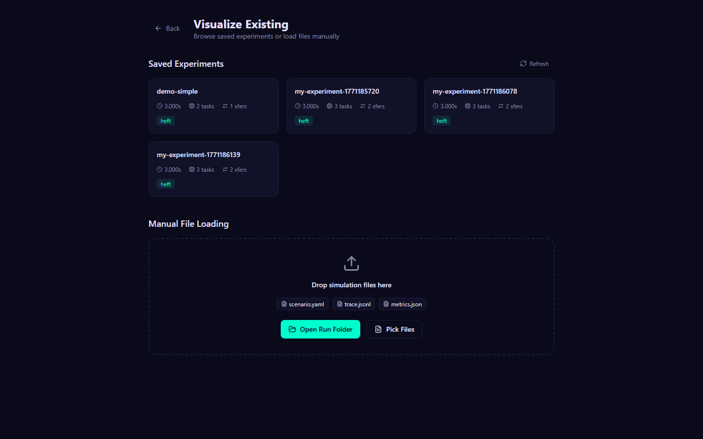
The experiment browser lists all saved experiments from the
viz/public/sample-runs/ directory. Each entry shows:
- Experiment name
- Scenario name
- Scheduler used
- Makespan result
Click any experiment to load it instantly. The same six visualization tabs become available with the loaded data.
Adding your own experiments
To add a CLI-generated experiment to the browser, copy its output
directory into viz/public/sample-runs/:
Refresh the browser to see it in the list.
Keyboard Shortcuts Reference
| Shortcut | Action |
|---|---|
| 1 through 6 | Switch between visualization tabs |
| Space | Play / Pause simulation playback |
| Right | Step forward one event |
| Left | Step backward one event |
| + | Increase playback speed |
| - | Decrease playback speed |
| Home | Jump to beginning of simulation |
| End | Jump to end of simulation |
| ? | Show keyboard shortcuts help |
Summary
You have now explored every feature of ncsim-viz:
- Home Page -- Choose between Configure & Run or Visualize Existing
- Configuration Form -- Build scenarios with topology, DAG, and interference settings
- Overview Tab -- Dashboard metrics and utilization bars
- Network Tab -- Interactive force-directed topology graph
- DAG Tab -- Hierarchical task dependency visualization
- Schedule Tab -- Static Gantt chart of the full execution timeline
- Simulation Tab -- Animated event replay with synchronized views
- Parameters Tab -- Read-only configuration inspector
- Experiment Browser -- Load and compare saved experiments
Next Steps
- Viz Setup -- Installation details for the viz platform
- Visualization Tabs -- Detailed reference for each tab
- Keyboard Shortcuts -- Complete shortcut reference
- Tutorial 4: Compare Schedulers -- Generate results to visualize
Reference
FAQ
Frequently asked questions about ncsim, organized by topic.
General
Q: What is ncsim?
A: ncsim is a headless discrete-event simulator for evaluating task scheduling algorithms on heterogeneous networked computing systems. It models compute nodes with different capacities, network links with bandwidth sharing and WiFi interference, and DAG-structured task graphs with data dependencies.
Q: Who develops ncsim?
A: ncsim is developed by the Autonomous Networks Research Group (ANRG) at the University of Southern California. Contributors: Bhaskar Krishnamachari, Maya Gutierrez.
Q: Is ncsim free to use?
A: Yes. ncsim is open source under the MIT license. You can use, modify, and distribute it freely.
Q: What Python version is required?
A: Python 3.10 or later. Check your version with python --version.
Q: How do I cite ncsim?
A: See the CITATION.cff file in the repository root for the
recommended citation format. The repository also has a Zenodo DOI for
versioned citations.
Simulation
Q: Is the simulation deterministic?
A: Yes. Given the same inputs (scenario YAML) and the same seed
(--seed), ncsim produces identical event sequences and results every
time. This determinism is guaranteed by:
- Microsecond time precision (6 decimal places) to prevent floating-point drift
- Deterministic event ordering via
(time, priority, insertion_id)tuples in the priority queue - Seeded random number generation for stochastic elements like shadow fading
Verify determinism
Run the same scenario twice with the same seed and diff the traces:
ncsim --scenario scenarios/demo_simple.yaml --output out/a --seed 42
ncsim --scenario scenarios/demo_simple.yaml --output out/b --seed 42
diff out/a/trace.jsonl out/b/trace.jsonl
The diff should produce no output.
Q: What does "makespan" mean?
A: Makespan is the total simulation time from the start of the first task to the completion of the last task. It is the primary performance metric for comparing scheduling algorithms. Lower is better.
Q: Can I simulate multiple DAGs?
A: Yes. The YAML format supports multiple DAGs under the dags: section.
Each DAG has its own inject_at time, allowing you to model workflows
that arrive at different points during the simulation.
dags:
- id: dag_1
inject_at: 0.0
tasks: [...]
edges: [...]
- id: dag_2
inject_at: 5.0
tasks: [...]
edges: [...]
Q: What units are used throughout ncsim?
A: All units are consistent across the simulator:
| Quantity | Unit |
|---|---|
| Compute capacity | units per second |
| Compute cost | units (runtime = cost / capacity) |
| Bandwidth | MB/s |
| Latency | seconds |
| Data size | MB |
| Positions | meters (x, y coordinates) |
| Makespan / duration | seconds |
| Transmit power | dBm |
| Frequency | GHz |
| Noise floor | dBm |
| CCA threshold | dBm |
Q: How does bandwidth sharing work?
A: When N data transfers share a single link simultaneously, each
transfer receives bandwidth / N of the link's effective bandwidth.
Transfer completion times are recalculated dynamically whenever a new
transfer starts or an existing transfer completes on the same link.
For example, on a 100 MB/s link:
- 1 transfer: 100 MB/s each
- 2 concurrent transfers: 50 MB/s each
- 3 concurrent transfers: 33.3 MB/s each
This fair-sharing model stacks with the interference factor:
Q: What happens when a task has no predecessors?
A: Tasks with no incoming edges are considered entry tasks. They become
ready for execution as soon as their DAG is injected (at the inject_at
time). If the assigned node is idle, execution starts immediately.
Scheduling
Q: Which scheduler should I use?
A: Use HEFT as the default. It is the best general-purpose scheduling algorithm in ncsim:
| Situation | Recommended Scheduler |
|---|---|
| General purpose | HEFT |
| Dominant critical path + one fast node | CPOP |
| Baseline comparison | Round Robin |
| Controlled experiment with fixed placement | Manual (pinned_to) |
See the Scheduling Concepts page for a detailed comparison.
Q: What does pinned_to do?
A: The pinned_to field in a task definition forces that task to run on
a specific node, overriding the scheduler's placement decision. It works
with all schedulers:
This is useful for controlled experiments where you want to test a specific placement, or for modeling tasks that must run on particular hardware.
Q: What happens if anrg-saga is not installed?
A: If the anrg-saga package is not available, ncsim cannot use the HEFT
or CPOP schedulers. It falls back to Round Robin with a warning. Install
anrg-saga to restore HEFT and CPOP support:
WiFi and Interference
Q: When should I use csma_bianchi vs csma_clique?
A: Choose based on the level of realism you need:
| Model | Realism | Dynamic | Best For |
|---|---|---|---|
csma_bianchi |
High | Yes (recalculates per transfer) | Research-quality results, realistic WiFi |
csma_clique |
Medium | No (static worst-case) | Quick WiFi-aware approximation |
csma_bianchi is more realistic because it dynamically separates
contention domain time-sharing (Bianchi MAC efficiency) from hidden
terminal SINR degradation. csma_clique applies a static worst-case
bandwidth reduction based on the maximum clique size.
Performance consideration
csma_bianchi recalculates interference factors whenever any
transfer starts or completes, which adds computational overhead for
large networks. csma_clique computes bandwidth once at setup time
and never recalculates.
Q: What happens if WiFi links have no explicit bandwidth?
A: When using csma_clique or csma_bianchi, links without a
bandwidth field in the YAML derive their data rate from the RF model:
- Node positions determine distance
- Distance determines path loss
- Path loss determines received power and SNR
- SNR selects the highest viable MCS rate
- MCS rate becomes the link's PHY bandwidth (in MB/s)
This allows you to define a topology with only positions and RF parameters, and let the WiFi model compute realistic bandwidths automatically.
Q: Can I mix wired and wireless links?
A: Yes. Links with an explicit bandwidth field in the YAML keep their
specified value -- the WiFi model does not overwrite it. Links without
a bandwidth field use the WiFi-derived rate. This allows you to model
mixed wired/wireless scenarios:
links:
- id: ethernet_link
from: server
to: switch
bandwidth: 1000 # 1 GB/s wired -- kept as-is
latency: 0.0001
- id: wifi_link
from: switch
to: laptop
latency: 0.001
# No bandwidth -- derived from RF model
Q: What is the conflict graph?
A: The conflict graph determines which links cannot transmit simultaneously under the CSMA/CA protocol. Two links conflict if one transmitter's signal is strong enough to trigger the other's carrier sensing mechanism. The maximum clique size in this graph determines worst-case contention. See the WiFi Model page for details.
Q: Does RTS/CTS change the results?
A: Yes. Enabling RTS/CTS (--rts-cts flag) extends the conflict zone
to protect receivers, not just transmitters. This increases the number
of conflicting links (larger cliques) but reduces hidden terminal
problems. The net effect depends on the topology -- in some cases
RTS/CTS improves throughput by preventing hidden terminal interference;
in others it reduces throughput by increasing contention.
Visualization
Q: Do I need the viz to use ncsim?
A: No. The CLI (ncsim command) is fully self-contained. It reads a
scenario YAML, runs the simulation, and writes trace.jsonl,
metrics.json, and a copy of the scenario to the output directory. The
viz is an optional tool for interactive configuration, visual analysis,
and animated replay.
Q: Can I use the viz without the backend?
A: Partially. The "Visualize Existing" mode can load pre-generated
sample runs from viz/public/sample-runs/ without the backend if the
files are served as static assets. However, the experiment list API
(/api/experiments) requires the backend, and "Configure & Run" mode
always requires the backend to execute simulations.
Q: What browsers are supported?
A: ncsim-viz is tested on modern versions of Chrome, Firefox, Safari, and Edge. It requires JavaScript enabled and works best with hardware acceleration for the D3 visualizations.
Q: Can I export visualizations as images?
A: The current version does not have a built-in export feature. You can use your browser's screenshot tools or the developer console to capture visualizations. The Gantt chart and network graph are rendered as SVG elements that can be extracted.
Output Files
Q: What files does each simulation run produce?
A: Every run writes three files to the --output directory:
| File | Format | Contents |
|---|---|---|
scenario.yaml |
YAML | Copy of the input scenario (for reproducibility) |
trace.jsonl |
JSON Lines | Every simulation event, one JSON object per line |
metrics.json |
JSON | Summary metrics: makespan, utilization, counts |
See the Output Files reference for detailed field descriptions.
Q: Can I load trace files from the CLI into the viz?
A: Yes. Copy the output directory (containing scenario.yaml,
trace.jsonl, and metrics.json) into viz/public/sample-runs/ and
it will appear in the experiment browser. You can also use the file
loader to upload individual files directly.
Troubleshooting
Solutions for common issues encountered when installing, running, or visualizing ncsim simulations.
Installation Issues
ModuleNotFoundError: No module named 'ncsim'
Cause: ncsim is not installed in the active Python environment.
Fix: Install ncsim in editable mode from the repository root:
If you are using a virtual environment, make sure it is activated first:
# Linux / macOS
source venv/bin/activate
# Windows
venv\Scripts\activate
# Then install
pip install -e .
ncsim: command not found
Cause: The pip scripts directory is not on your system PATH.
Fix: Use python -m ncsim as an alternative, or add pip's bin
directory to your PATH:
# Option A: Run as a module (always works)
python -m ncsim --scenario scenarios/demo_simple.yaml --output results/test
# Option B: Find the scripts directory
python -m site --user-base
# Add the bin/ (Linux/macOS) or Scripts/ (Windows) subdirectory to PATH
ImportError: anrg-saga
Cause: The anrg-saga package is not installed, or a conflicting
saga package is present.
Fix: Install or upgrade anrg-saga:
If you have a different package named saga installed, uninstall it
first:
pygraphviz on Windows
The anrg-saga package has an optional dependency on pygraphviz,
which can be difficult to install on Windows. If the full install
fails, install without optional dependencies:
SAGA library not available (warning at runtime)
Cause: The anrg-saga package is not importable, so HEFT and CPOP
schedulers are unavailable.
Fix: Reinstall anrg-saga:
When SAGA is unavailable, ncsim falls back to Round Robin scheduling with a warning. HEFT and CPOP will not be available until SAGA is properly installed.
pip install -e . fails with build errors
Cause: Missing build dependencies or incompatible Python version.
Fix:
- Verify Python version is 3.10+:
python --version - Upgrade pip and setuptools:
pip install --upgrade pip setuptools - Retry:
pip install -e .
CLI Issues
"to_node 'X' not found"
Cause: A link in the scenario YAML references a node ID that does
not exist in the nodes: list.
Fix: Open the scenario YAML and verify that every from: and to:
value in the links: section matches an id: in the nodes: section.
nodes:
- id: n0 # <-- node IDs defined here
- id: n1
links:
- id: l01
from: n0 # <-- must match a node ID above
to: n1 # <-- must match a node ID above
No direct link between nodes
Cause: The scheduler assigned communicating tasks to nodes that are
not directly connected, but direct routing is active.
Fix: Switch to multi-hop routing:
Or use --routing shortest_path. Both support multi-hop data transfers
through intermediate relay nodes.
Why this happens
HEFT and CPOP choose node assignments based on compute speed and may place dependent tasks on non-adjacent nodes. Direct routing only works when every communicating pair has an explicit link. Multi-hop routing resolves this by forwarding data through intermediate nodes.
Simulation takes very long
Cause: Large networks with the csma_bianchi interference model.
Bianchi recalculates interference factors for all active links whenever
any transfer starts or completes.
Fix: Several options, in order of preference:
-
Use
csma_cliqueinstead -- computes bandwidth once at setup, no dynamic recalculation: -
Reduce network size -- fewer links means fewer recalculations.
-
Use
proximityinterference -- simpler distance-based model: -
Disable interference entirely -- for wired networks or when interference is not relevant:
Invalid scheduler / routing / interference value
Cause: Unrecognized value passed to --scheduler, --routing, or
--interference.
Fix: Use one of the supported values:
| Flag | Valid Values |
|---|---|
--scheduler |
heft, cpop, round_robin, manual |
--routing |
direct, widest_path, shortest_path |
--interference |
none, proximity, csma_clique, csma_bianchi |
Unexpected makespan (all schedulers produce the same result)
Cause: All tasks have pinned_to set, which overrides the
scheduler's placement decisions.
Fix: If you want the scheduler to make placement decisions, remove
the pinned_to fields from the task definitions in the scenario YAML.
Visualization Issues
Frontend shows "Network Error" on Run
Cause: The FastAPI backend is not running, or there is a CORS / proxy configuration issue.
Fix:
-
Verify the backend is running:
-
Check the terminal for error messages (missing modules, port conflicts).
-
Ensure you are accessing the frontend at
http://localhost:5173(not port 8000 directly). The Vite proxy forwards/api/*requests to the backend.
Port 8000 or 5173 already in use
Cause: Another process is occupying the required port.
Fix: Find and stop the conflicting process:
Alternatively, change the port:
# Backend on a different port
cd viz/server
uvicorn main:app --port 8001
# Frontend on a different port
cd viz
npx vite --port 3000
Proxy configuration
If you change the backend port, update the proxy setting in
viz/vite.config.ts to match the new port.
npm install fails
Cause: Node.js version is too old. The frontend requires Node.js 18 or later.
Fix: Upgrade Node.js:
# Check current version
node --version
# Upgrade (using nvm)
nvm install 18
nvm use 18
# Or download from https://nodejs.org/
# Retry installation
cd viz
npm install
Viz shows no experiments in browser
Cause: The viz/public/sample-runs/ directory is missing or does
not contain any experiment results.
Fix: Run a simulation and copy the output to the sample-runs directory:
# Run a simulation
ncsim --scenario scenarios/demo_simple.yaml --output results/demo
# Copy to sample-runs
cp -r results/demo viz/public/sample-runs/demo
Then refresh the browser. The experiment should appear in the list.
Visualization is slow or unresponsive
Cause: Very large traces (thousands of events) can slow down the D3 visualizations.
Fix:
- Use a smaller scenario for interactive exploration.
- For large experiments, use the CLI analysis tools (
analyze_trace.py) instead of the web UI. - Ensure hardware acceleration is enabled in your browser settings.
Common Errors Reference Table
| Error | Cause | Fix |
|---|---|---|
ModuleNotFoundError: ncsim |
Not installed | pip install -e . |
ncsim: command not found |
PATH issue | Use python -m ncsim |
ImportError: anrg-saga |
Missing dependency | pip install "anrg-saga>=2.0.3" |
"to_node 'X' not found" |
Invalid node reference in YAML | Check that all link endpoints match node IDs |
No direct link |
Direct routing + non-adjacent nodes | Use --routing widest_path |
Network Error in viz |
Backend not running | Start python run.py on port 8000 |
Port in use |
Port conflict | Kill conflicting process or change port |
npm install fails |
Old Node.js | Upgrade to Node.js 18+ |
SAGA not available |
anrg-saga not importable | pip install "anrg-saga>=2.0.3" |
| Same makespan for all schedulers | All tasks have pinned_to |
Remove pinned_to to let scheduler decide |
Getting More Help
If your issue is not covered here:
-
Enable verbose logging to get detailed debug output:
-
Check the trace file (
trace.jsonl) for unexpected event sequences. -
Review the metrics file (
metrics.json) for error messages in theerror_messagefield. -
File an issue on the GitHub repository with:
- The scenario YAML file
- The full error message or unexpected output
- Your Python version (
python --version) - Your ncsim version (
ncsim --version)
Glossary
Alphabetical reference of key terms used throughout the ncsim documentation and codebase.
B
- Bandwidth
- Data transfer rate of a network link, measured in MB/s. When multiple transfers share a link, each receives an equal fraction of the available bandwidth. Bandwidth may be reduced by interference models.
- Bianchi Model
- Analytical model for IEEE 802.11 DCF MAC throughput, derived by
Giuseppe Bianchi (2000). Computes the MAC efficiency
eta(n)forncontending stations by solving coupled equations for transmission probability and collision probability. Used by thecsma_bianchiinterference model.
C
- CCA (Clear Channel Assessment)
- Mechanism by which a WiFi node determines whether the wireless channel is currently busy. A node detects the channel as busy when the received signal power exceeds the CCA threshold (default: -82 dBm). CCA determines the carrier sensing range and therefore the conflict graph.
- Clique
- A set of nodes (links) in the conflict graph where every pair is
connected by an edge -- meaning every pair conflicts. The maximum
clique size containing a given link determines the worst-case
number of contenders. Used by both
csma_cliqueandcsma_bianchiinterference models. - Compute Capacity
- Processing speed of a node, measured in compute units per second.
A node with capacity 100 completes a task with cost 200 in
200 / 100 = 2.0seconds. - Compute Cost
- Total work required by a task, measured in compute units. The
runtime on a given node is
compute_cost / compute_capacity. - Conflict Graph
- An undirected graph where vertices represent network links and
edges connect pairs of links that cannot transmit simultaneously
due to carrier sensing. Built from node positions and RF parameters.
The conflict graph is used by both
csma_cliqueandcsma_bianchiinterference models to determine contention relationships. - CPOP (Critical Path on a Processor)
- A list-scheduling algorithm that identifies the DAG's critical path
and assigns all critical-path tasks to the single processor that
minimizes their total execution time. Non-critical tasks are assigned
using the Earliest Finish Time heuristic. Implemented via the
anrg-sagalibrary.
D
- DAG (Directed Acyclic Graph)
- A task dependency graph where vertices represent tasks and directed edges represent data dependencies. A task cannot start until all its predecessor tasks have completed and all required data transfers have finished. ncsim supports multiple DAGs injected at different times.
- DES (Discrete Event Simulation)
- A simulation paradigm where the system state changes only at discrete time points called events. Between events, the system state is constant. ncsim uses DES with a priority queue to process events in chronological order.
E
- EFT (Earliest Finish Time)
- The earliest time at which a task can complete on a given node, accounting for the task's computation time, all required data transfer times from predecessor tasks, and the node's current availability. Used by HEFT and CPOP for node selection.
- Event Queue
- A priority queue that orders simulation events by a tuple of
(time, priority, insertion_id). The time determines chronological order. The priority breaks ties between events at the same time. The insertion ID breaks remaining ties to ensure deterministic, stable ordering.
- HEFT (Heterogeneous Earliest Finish Time)
- The default scheduling algorithm in ncsim. A list-scheduling
heuristic that sorts tasks by decreasing upward rank and assigns
each task to the node that minimizes the Earliest Finish Time.
Communication-aware and heterogeneity-aware. Implemented via the
anrg-sagalibrary. - Hidden Terminal
- A transmitter that is outside the carrier sensing range of another
transmitter but whose signal can still cause interference at the
other link's receiver. Hidden terminals affect SINR but are not
prevented by CSMA. The
csma_bianchimodel explicitly accounts for hidden terminal degradation.
I
- Interference Factor
- A multiplicative factor in the range (0, 1] applied to a link's base bandwidth due to wireless interference from other active links. An interference factor of 0.5 means the link operates at half its nominal bandwidth. The factor is computed by the active interference model and stacks with per-link fair sharing.
L
- Latency
- Propagation delay on a network link, measured in seconds. For
multi-hop routes, latencies are summed across all hops
(store-and-forward model). Total transfer time is
(data_size / bandwidth) + latency. - Link
- A directed communication channel between two nodes. Defined by a
source node (
from), destination node (to), bandwidth (MB/s), and latency (seconds). Multiple concurrent transfers on the same link share its bandwidth equally.
M
- Makespan
- Total time from the start of the first task to the completion of the last task across all DAGs. The primary performance metric for comparing scheduling algorithms and configurations. Lower makespan indicates better performance.
- MCS (Modulation and Coding Scheme)
- A WiFi PHY layer encoding that determines the data rate achievable at a given SNR level. Higher MCS indices use denser modulation (e.g., 256-QAM, 1024-QAM) for higher rates but require stronger signals. ncsim includes MCS tables for 802.11n, 802.11ac, and 802.11ax.
- Metrics
- Summary statistics written to
metrics.jsonafter each simulation run. Includes makespan, total task and transfer counts, per-node utilization, per-link utilization, and (for WiFi models) RF configuration details and PHY rates. - Multi-hop
- Routing data through one or more intermediate relay nodes when no
direct link exists between the source and destination. Enabled by
widest_pathorshortest_pathrouting. Intermediate nodes act as store-and-forward relays.
N
- Node
- A compute resource in the network. Each node has an ID, a compute capacity (units/second), and optionally a position (x, y in meters). Tasks are scheduled onto nodes by the scheduling algorithm.
P
- Path Loss
- Signal attenuation as a function of distance. ncsim uses the
log-distance path loss model with a Friis free-space reference at
1 meter:
PL(d) = PL(d0) + 10 * n * log10(d / d0), wherenis the path loss exponent. - PHY Rate
- Physical layer data rate determined by MCS selection based on the
received SNR (or SINR under interference). Measured in Mbps and
converted to MB/s internally (
rate_MBps = rate_Mbps / 8). Scales linearly with channel width. - Placement Plan
- The output of a scheduling algorithm: a mapping from every task ID to a node ID. The placement plan determines where each task will execute. The execution engine then determines when each task runs based on event ordering and node availability.
- Position
- Physical location of a node as an
(x, y)coordinate pair in meters. Used for interference calculations (distance-based path loss, carrier sensing range) and for node placement in the visualization.
R
- RTS/CTS (Request to Send / Clear to Send)
- An optional 802.11 handshake protocol that extends the conflict
graph to protect receivers, not just transmitters. When enabled
(
--rts-cts), any node of link A sensing any node of link B causes a conflict. This reduces hidden terminal problems but increases contention.
S
- Scenario
- A complete simulation specification in YAML format. Contains the network definition (nodes and links), one or more DAGs (tasks and edges), and configuration options (scheduler, routing, interference, seed, RF parameters).
- Seed
- A random seed integer for deterministic simulation reproducibility.
The same scenario with the same seed always produces identical
results. Set via
--seedon the CLI orseed:in the YAML config. - Shadow Fading
- Random signal variation modeled as a log-normal distribution
N(0, sigma)in the dB domain. Each node pair receives a deterministic fading value (symmetric and seeded). Configured viashadow_fading_sigma(default: 0.0, meaning no fading). - SINR (Signal-to-Interference-plus-Noise Ratio)
- The ratio of desired signal power to the sum of interference power and noise power, measured in dB. Determines the achievable data rate under interference from hidden terminals. Lower SINR may force a lower MCS selection and reduced throughput.
- SNR (Signal-to-Noise Ratio)
- The ratio of received signal power to noise floor power, measured in
dB:
SNR = Prx - N0. Determines the achievable data rate in the absence of interference. Used for MCS rate selection.
T
- Task
- A unit of computation with a compute cost, scheduled onto a node by the scheduling algorithm. Tasks may have data dependencies (edges in the DAG) that require transfers to complete before execution can begin.
- Trace
- The event log written to
trace.jsonlafter each simulation run. Contains one JSON object per line, recording every discrete event in chronological order. Events include simulation start/end, DAG injection, task scheduling/start/completion, and transfer start/completion.
U
- Upward Rank
- A metric used by HEFT to prioritize tasks. Defined as the longest path (by computation + communication cost) from a task to any exit task in the DAG. Tasks with higher upward rank are scheduled first, ensuring that critical-path tasks receive priority.
- Utilization
- The fraction of the makespan during which a resource (node or link)
was actively working. Node utilization measures compute time; link
utilization measures transfer time. Reported as a value between 0.0
(idle) and 1.0 (fully utilized) in
metrics.json.
W
- Widest Path
- A routing strategy that finds the path between two nodes that maximizes the bottleneck (minimum) bandwidth along the path. Uses a modified Dijkstra algorithm with a max-heap. Optimal for large data transfers where bandwidth dominates transfer time.
Y
- YAML
- YAML Ain't Markup Language. A human-readable data serialization format used for ncsim scenario files. Scenario YAML files define the network topology, DAG task graphs, and simulation configuration. See the YAML Reference for the complete format specification.