Tutorial 5: Visualization Walkthrough
A click-by-click tour of the Ncsim 1.1.0 visualization UI, including the full SAGA 2.1 scheduler catalog, RF-derived link rates, experiment execution, and all six result tabs.
All screenshots in this tutorial were captured from the current visualization UI in light mode at 1440 x 900 with SAGA 2.1.0 installed.
What You Will Learn
- Start the visualization backend and frontend
- Select any installed SAGA scheduler and set supported constructor options
- Configure topology, DAG, routing, interference, and RF-derived link rates
- Run an experiment from the browser
- Explore all six result tabs
- Browse saved runs or load result files manually
- Use the visualization keyboard shortcuts
Prerequisites
| Requirement | Version / Command |
|---|---|
| Ncsim | Install from the repository with pip install -e . |
| SAGA | 2.1.0 tagged source release for the 23-algorithm catalog |
| Backend | Python 3.12+, FastAPI, and Uvicorn |
| Frontend | Node.js 18+ and npm install in viz/ |
Install the visualization dependencies from the repository root:
pip install -e .
python -m pip install "anrg-saga @ git+https://github.com/ANRGUSC/saga.git@v2.1.0"
pip install -r viz/server/requirements.txt
cd viz
npm install
cd ..
Step 1: Start Ncsim-Viz
GitHub Codespaces
The current repository includes a start-viz helper. From the repository root:
Open the forwarded Ncsim visualization URL shown by Codespaces.
Local Development
Use two terminals.
Both servers are required for Configure & Run and for the saved-experiment browser. Manual file loading can render results in the frontend without invoking the simulation API.
Step 2: Choose a Workflow
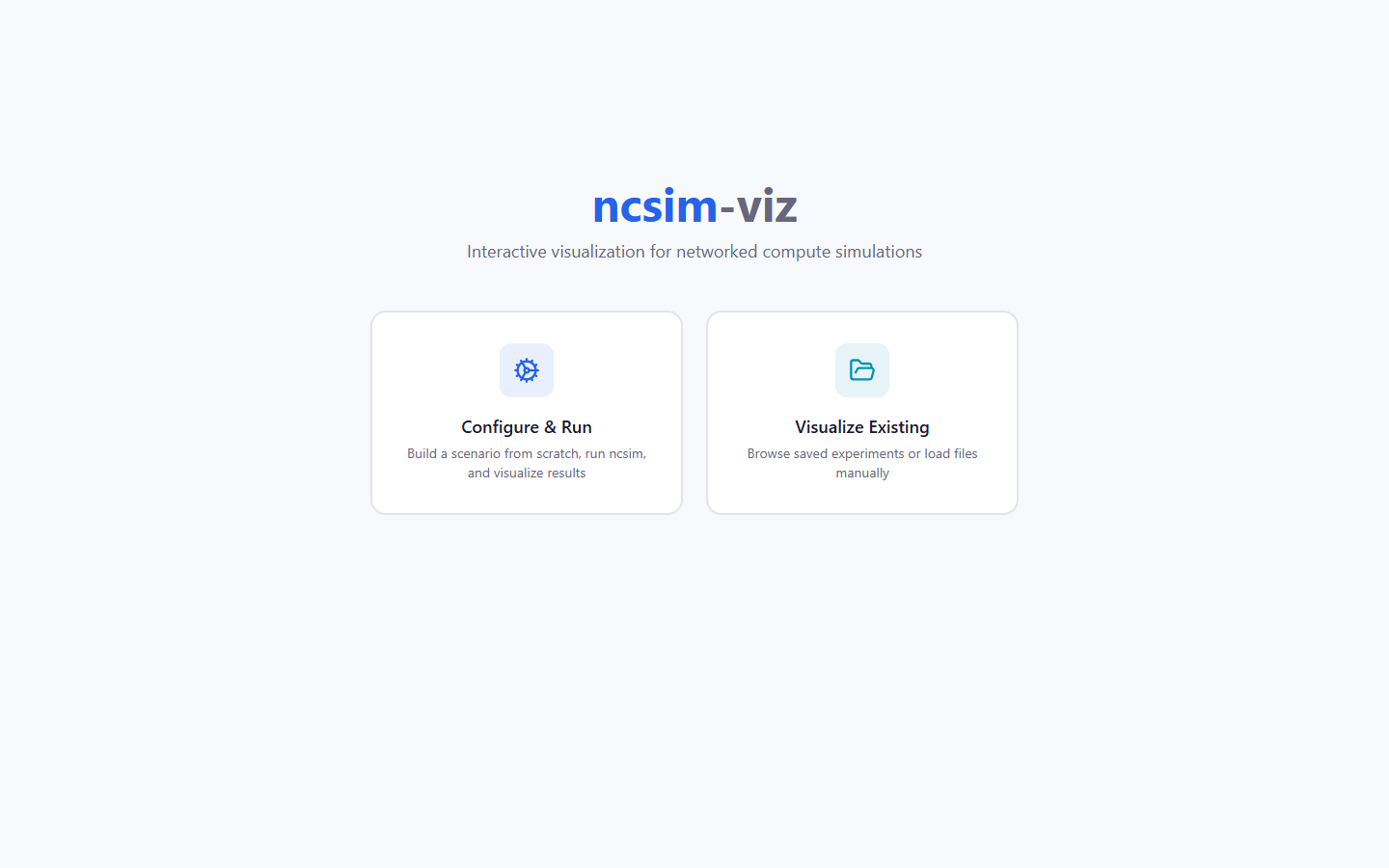
The home page offers two workflows:
| Workflow | Purpose |
|---|---|
| Configure & Run | Build a scenario, execute Ncsim through the backend, and open the results immediately |
| Visualize Existing | Browse saved runs or load scenario.yaml, trace.jsonl, and metrics.json from disk |
Click Configure & Run.
Step 3: Set the Basic Configuration
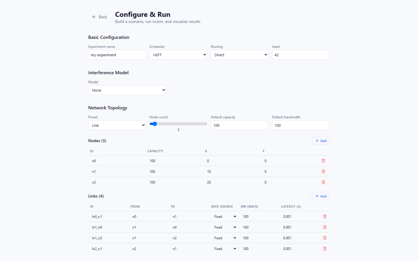
The form starts with these defaults:
| Field | Default | Meaning |
|---|---|---|
| Experiment name | my-experiment |
Slug used for the saved run directory |
| Scheduler | HEFT | Task-to-node placement algorithm |
| Routing | Direct | Route model used for inter-node transfers |
| Seed | 42 | Reproducibility seed |
| Interference | None | No inter-link interference adjustment |
The scheduler selector is populated by the backend's /api/schedulers endpoint.
With SAGA 2.1 installed, it contains 23 SAGA algorithms plus the built-in
Round Robin and Manual choices.
If SAGA 2.0.4 is installed instead, the selector contains 22 SAGA algorithms and omits PEFT; the UI always reflects the backend's installed scheduler catalog.
Scheduler Options
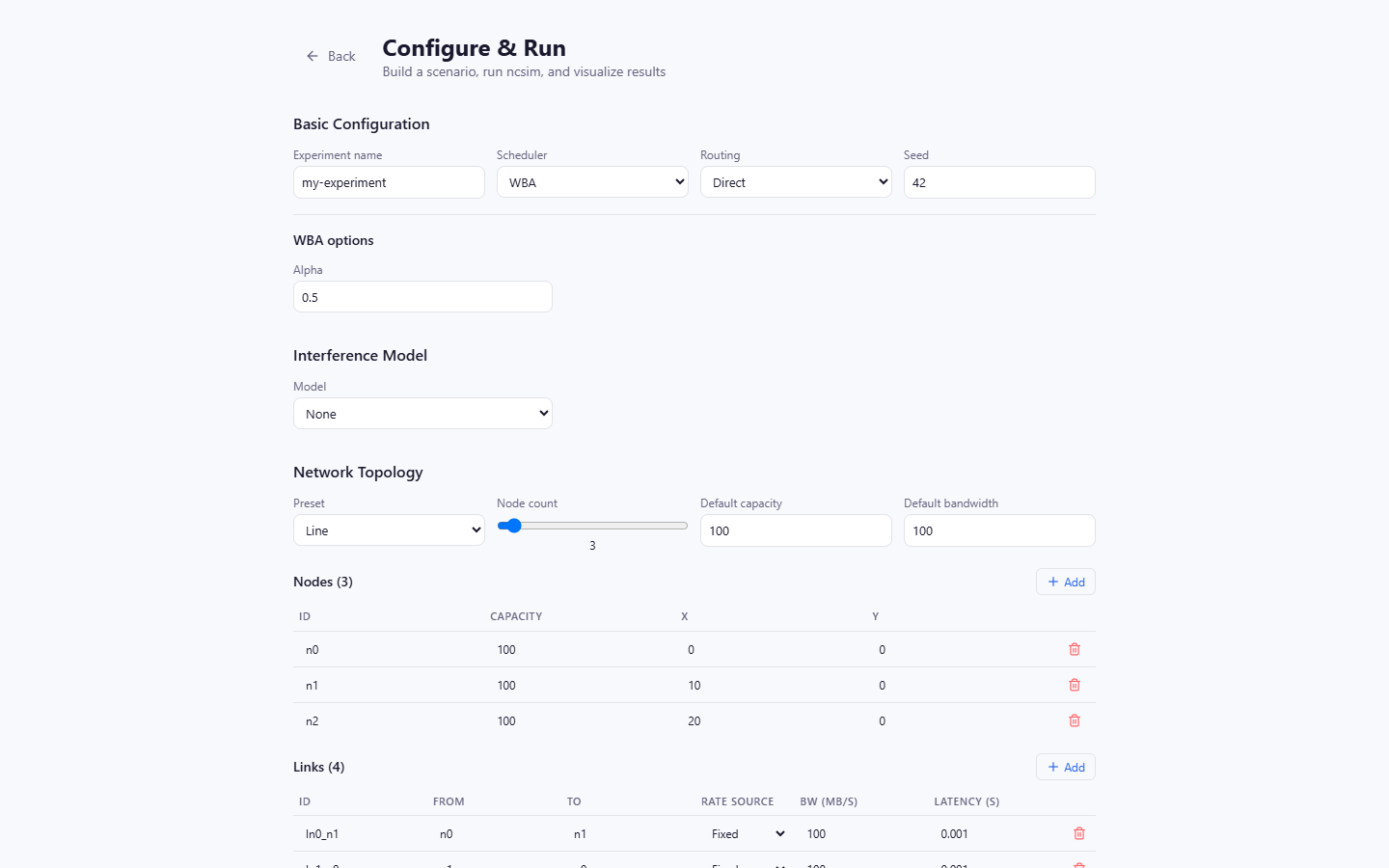
When a scheduler exposes constructor settings, typed controls appear below the selector:
| Scheduler | UI Option |
|---|---|
| FCP | Priority queue size |
| GDL | Dynamic level (1 or 2) |
| SMT | Epsilon and optional solver name |
| WBA | Alpha (0 to 1) |
The generated YAML stores these values in config.scheduler_options. Select
HEFT again before continuing.
Step 4: Build a Network Topology
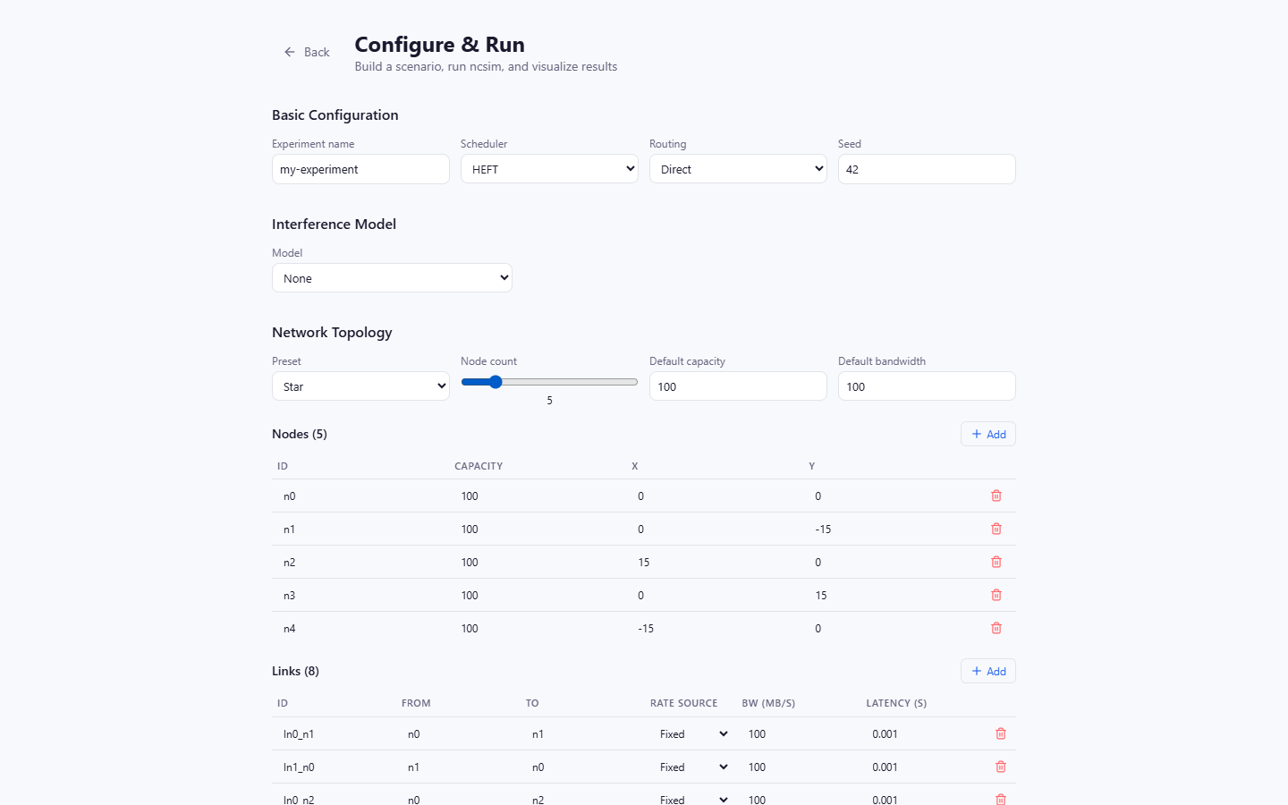
Select the Star preset and set Node count to 5. Current topology
presets are:
- Line
- Ring
- Star
- Mesh (fully connected)
- Grid
- Random (radio-range)
- Custom
Every generated node and link remains editable. The random preset uses the seed and RF configuration to place nodes and connect pairs within radio range.
Each link has a Rate source:
| Rate Source | Behavior |
|---|---|
| Fixed | Use the explicit bandwidth value in MB/s |
| Auto (default) | Omit bandwidth and let the non-WiFi path use Ncsim's default |
| Auto (RF) | With csma_clique or csma_bianchi, omit bandwidth so Ncsim derives the PHY rate from distance and RF settings |
Step 5: Build a DAG
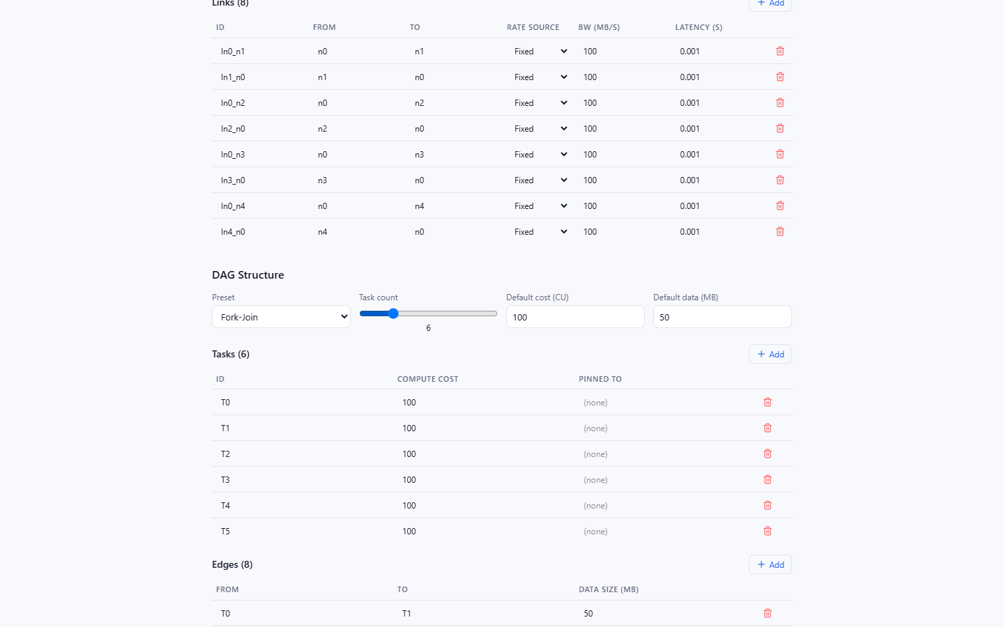
Select Fork-Join and set Task count to 6. The preset creates a source,
four parallel workers, and a sink. Other presets are Chain, Diamond, Parallel,
and Custom.
You can edit task IDs, compute costs, optional pinned_to assignments, edge
endpoints, and data sizes. When the Manual scheduler is selected, Pinned To
becomes a node dropdown; assign every task before running.
Step 6: Configure WiFi Interference
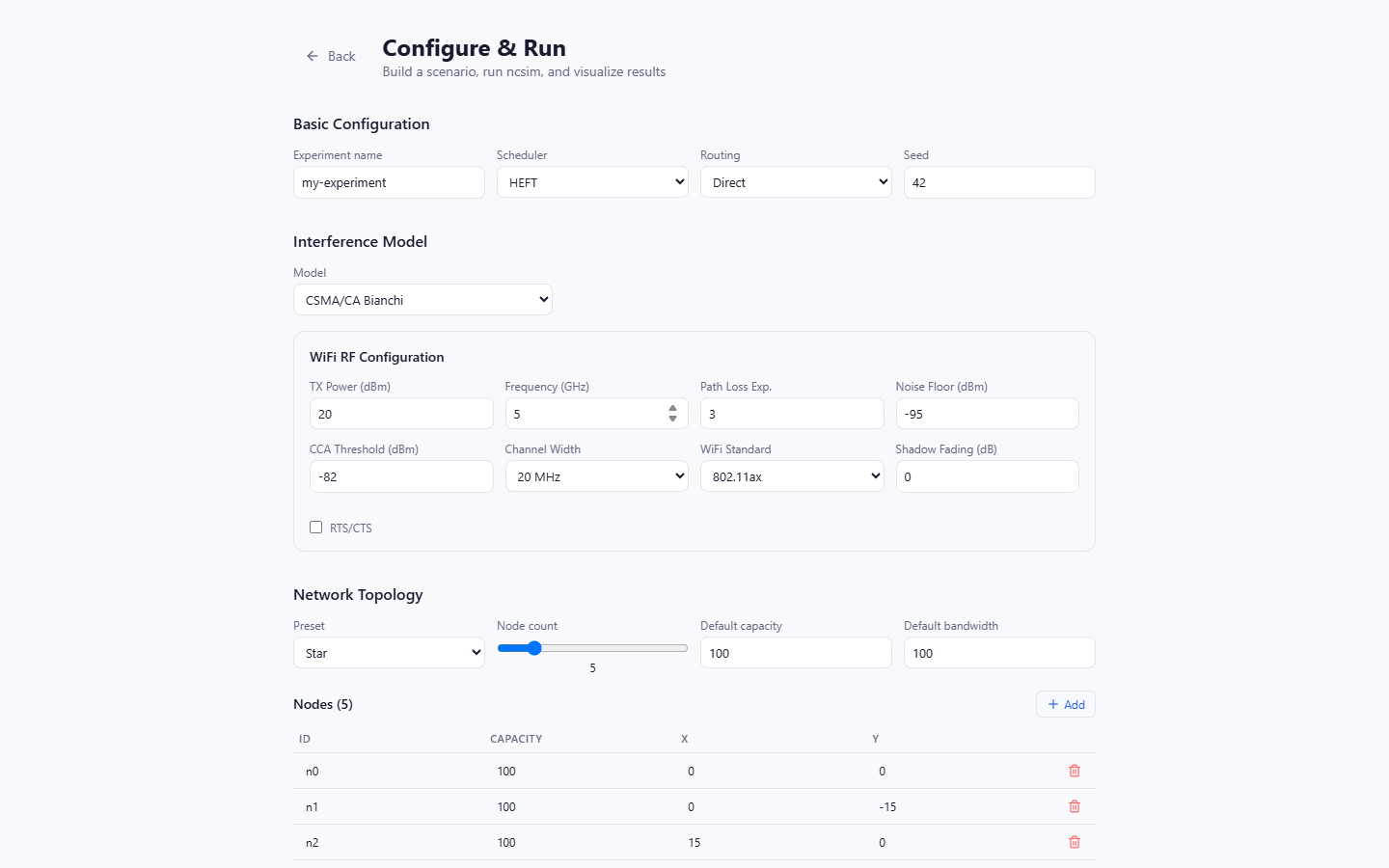
Select CSMA/CA Bianchi. The RF panel exposes:
- TX power and carrier frequency
- Path-loss exponent and noise floor
- CCA threshold and channel width
- WiFi standard (
802.11n,802.11ac, or802.11ax) - Shadow-fading sigma
- RTS/CTS
The four interference choices are:
| Model | Use |
|---|---|
| None | No inter-link interference model |
| Proximity | Fast radius-based bandwidth sharing approximation |
| CSMA/CA Clique | Static PHY-rate division by maximum conflict clique |
| CSMA/CA Bianchi | Dynamic WiFi contention with MAC efficiency and SINR effects |
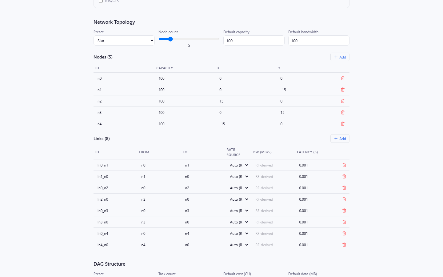
After selecting a WiFi model, choose Auto (RF) for links whose bandwidth should be derived from their node positions and the RF panel. Fixed links retain their entered bandwidth and are not overwritten in the generated YAML.
Step 7: Preview and Run
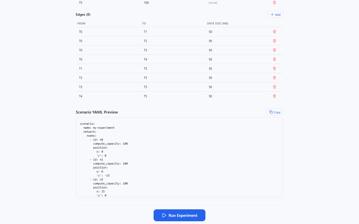
The YAML preview is live. Confirm that it contains:
- The scheduler and any
scheduler_options - Routing, seed, and interference model
- RF settings when a WiFi model is active
- Nodes, links, and fixed or omitted bandwidth fields
- Tasks, edges, and
pinned_tovalues
Click Run Experiment.
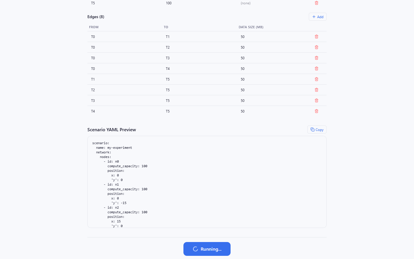
The backend writes the YAML to a temporary file, invokes the current Ncsim
package, and saves the completed run under viz/public/sample-runs/. The UI then
loads the returned scenario, trace, and metrics.
If the request fails, verify that port 8000 is serving the Ncsim FastAPI backend and inspect its terminal for a validation or scheduler error.
Step 8: Read the Overview
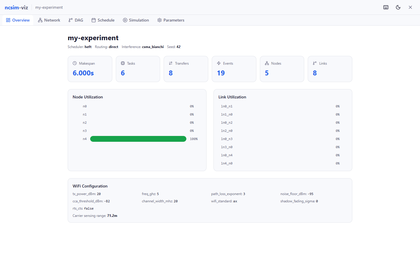
The Overview tab (1) summarizes:
- Makespan
- Task and transfer counts
- Node utilization
- Link utilization
- WiFi settings and derived rates when present
Utilization is normalized by makespan, making idle resources and hot spots easy to compare.
Step 9: Inspect the Network
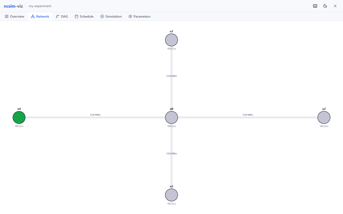
The Network tab (2) renders an interactive D3 topology.
- Drag nodes to reposition them
- Scroll to zoom and pan the SVG view
- Hover nodes for ID, compute capacity, and position
- Read link bandwidth and latency labels
Nodes are sized by compute capacity. In the simulation tab, active tasks and transfers use the same network layout.
Step 10: Inspect the DAG
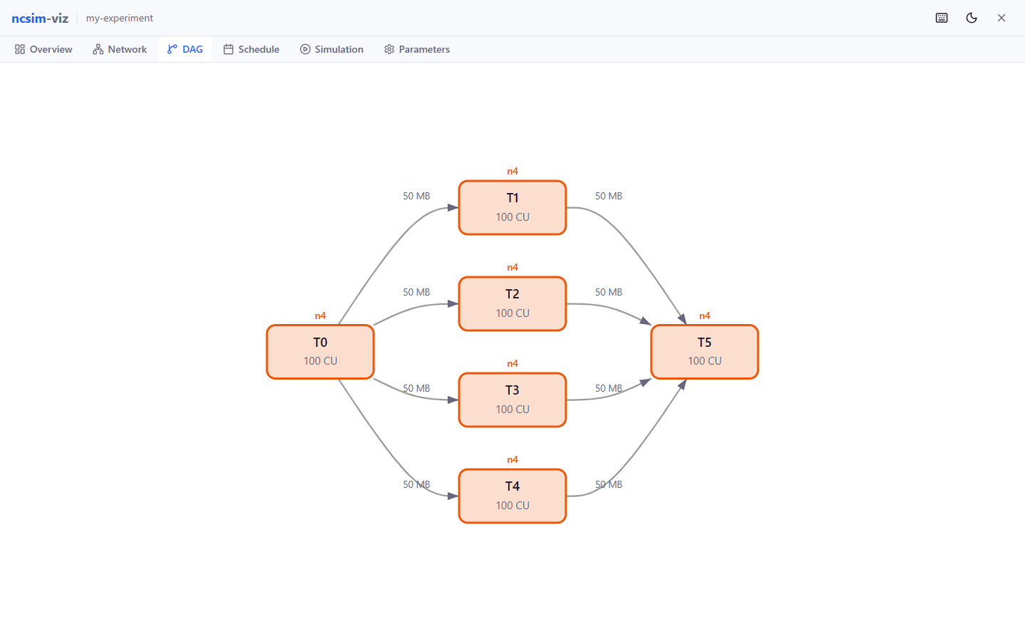
The DAG tab (3) uses a hierarchical Dagre layout. Tasks are colored by
their assigned compute node, while edges show dependency data sizes. Zoom or pan
the graph and hover a task for its assignment and timing details.
Step 11: Read the Schedule
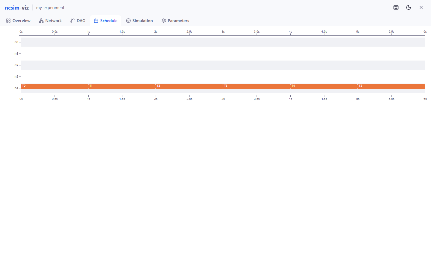
The Schedule tab (4) shows the complete execution timeline:
| Mark | Meaning |
|---|---|
| Solid task bar | Compute execution on a node |
| Transfer bar | Data movement on a link |
| Empty interval | Idle time |
Hover a bar for exact start, end, and duration values.
Step 12: Replay the Simulation
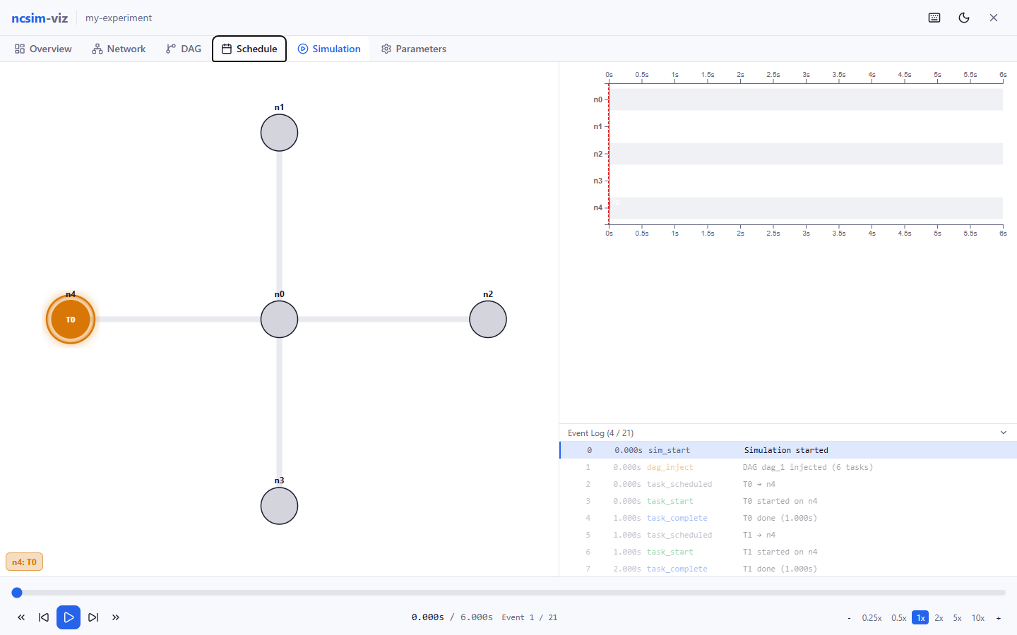
The Simulation tab (5) synchronizes three views:
- Network activity
- A growing Gantt timeline
- A clickable event log
Use the playback controls or keyboard:
| Shortcut | Action |
|---|---|
Space |
Play or pause |
Left / Right |
Step one event backward or forward |
Shift+Left / Shift+Right |
Jump 10% of the makespan |
Home / End |
Jump to the beginning or end |
+ / - |
Increase or decrease speed |
Clicking an event jumps directly to its simulation time.
Step 13: Verify the Parameters
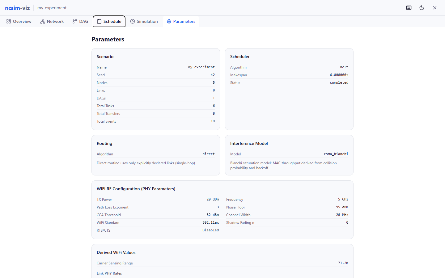
The Parameters tab (6) is the first place to check when a result is
surprising. It displays the scenario configuration, scheduler and routing,
network, DAG, task assignments, interference model, and RF values used by the
completed run.
Step 14: Browse or Load Existing Runs
Close the result view and select Visualize Existing.
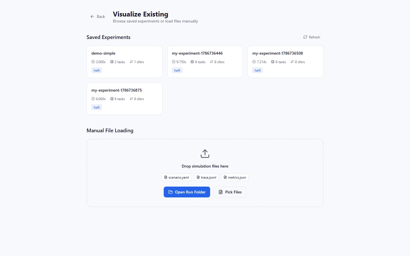
The browser lists directories under viz/public/sample-runs/ and shows available
makespan, task count, transfer count, and scheduler metadata. Click a card to open
the run.
You can also:
- Drop
scenario.yaml,trace.jsonl, andmetrics.jsontogether - Choose Open Run Folder
- Pick the three files individually
To expose a CLI-generated run in the saved-experiment browser:
Then click Refresh.
Keyboard Shortcuts
| Shortcut | Action |
|---|---|
1 through 6 |
Switch result tabs |
D |
Toggle dark or light mode |
? |
Open shortcut help |
Space |
Play or pause simulation replay |
Left / Right |
Step one replay event |
Shift+Left / Shift+Right |
Jump 10% |
Home / End |
Jump to start or end |
+ / - |
Change playback speed |
Summary
You have used the current Ncsim visualization workflow end to end:
- Started the API and frontend
- Loaded the installed 23-algorithm SAGA scheduler catalog
- Configured scheduler options, topology, DAG, routing, and interference
- Used fixed and RF-derived link rates
- Ran and saved an experiment
- Explored Overview, Network, DAG, Schedule, Simulation, and Parameters
- Browsed or manually loaded completed runs
Next Steps
- Tutorial 3: WiFi Experiment -- validate RF and interference behavior from the CLI
- Tutorial 4: Compare Schedulers -- run representative SAGA scheduler comparisons
- Visualization Tabs -- detailed tab reference
- Keyboard Shortcuts -- shortcut reference